bear this notice and the full citation on the first page. To copy otherwise, to ...
siders the worst-case, which usually does not translate to the average-case. To
us ...
Worst-Case Optimal and Average-Case Efficient ∗ Geometric Ad-Hoc Routing Fabian Kuhn, Roger Wattenhofer, Aaron Zollinger Department of Computer Science ETH Zurich 8092 Zurich, Switzerland {kuhn, wattenhofer, zollinger}@inf.ethz.ch
ABSTRACT
through a series of intermediate nodes—a process known as multi-hop routing. Routing is the foremost problem for mobile ad-hoc networks, thus it is not surprising that the research community has produced dozens of algorithmic proposals for routing [5, 11, 19, 21]. Why did researchers propose algorithms in such abundance? One possible answer to this question is that mobile ad-hoc networks have many parameters, such as transmission power, signal attenuation, interference, physical obstacles, type and extent of mobility, just to mention a few. Indeed with some parameters certain algorithms are superior to others, with some other parameters the ranking is reversed. It appears that a global evaluation is difficult. One way to cease the process of designing more and more hardly distinguishable algorithms is to assess the efficiency of the proposed algorithms by rigorous analysis. However, analyzing the complexity of mobile ad-hoc routing algorithms appears to be not only a demanding but an almost impossible mission. In order to come up with results, often worrisome assumptions that would never hold in practice need to be made. More important, analysis generally considers the worst-case, which usually does not translate to the average-case. To us only a few papers are known that analyze their algorithms analytically [2, 3, 4, 16, 18]. The method of choice to assess the average-case quality of an algorithm is simulation. A mobile ad-hoc network however having many parameters, simulation can never cover all the degrees of freedom. Some parameters are well-accepted: Nodes are considered to be points in a plane without obstructions, the nodes are equal in the sense that all of them have exactly the same radio and therefore the same transmission range. Other parameters are often questionable: Does it make sense that the nodes are distributed uniformly at random? In case the nodes are mobile, how do the nodes move? For the simulation part of our paper we use percolation theory to identify a critical network density range where routing is an inherently great challenge for any routing algorithm. We also observe that graphs generated at this critical density reflect reality more nicely than at higher densities; the “artificiality” introduced by placing nodes uniformly (although randomly) gains in importance with increasing network density only. We believe that our simulation guidelines are of value to any subsequent simulations in the area of multi-hop ad-hoc routing. We propose a new algorithm (dubbed GOAFR, Greedy Other Adaptive Face Routing, pronounced as “gopher”) for
In this paper we present GOAFR, a new geometric ad-hoc routing algorithm combining greedy and face routing. We evaluate this algorithm by both rigorous analysis and comprehensive simulation. GOAFR is the first ad-hoc algorithm to be both asymptotically optimal and average-case efficient. For our simulations we identify a network density range critical for any routing algorithm. We study a dozen of routing algorithms and show that GOAFR outperforms other prominent algorithms, such as GPSR or AFR.
Categories and Subject Descriptors F.2.2 [Analysis of Algorithms and Problem Complexity]: Nonnumerical Algorithms and Problems—geometrical problems and computations, routing and layout; C.2.2 [Computer-Communication Networks]: Network Protocols—routing protocols
General Terms Algorithms, Performance, Theory
Keywords Ad-Hoc Networks, Face Routing, Geometric Routing, Network Connectivity, Performance, Routing, Simulation, Wireless Communication
1.
INTRODUCTION
A mobile ad-hoc network consists of nodes equipped with wireless radio. For two nodes not in mutual transmission range to communicate, their messages need to be relayed ∗The work presented in this paper was supported (in part) by the National Competence Center in Research on Mobile Information and Communication Systems (NCCR-MICS), a center supported by the Swiss National Science Foundation under grant number 5005-67322.
Permission to make digital or hard copies of all or part of this work for personal or classroom use is granted without fee provided that copies are not made or distributed for profit or commercial advantage and that copies bear this notice and the full citation on the first page. To copy otherwise, to republish, to post on servers or to redistribute to lists, requires prior specific permission and/or a fee. MobiHoc’03, June 1–3, 2003, Annapolis, Maryland, USA. Copyright 2003 ACM 1-58113-684-6/03/0006 ...$5.00.
267
gle approach (introduced as Compass Routing in [16]) have been shown to fail on special graphs. Message delivery was guaranteed for the first time with Face Routing introduced in [16] (called Compass Routing II there). Face Routing walks along faces of planar graphs and proceeds along the line connecting the source and the destination. Besides guaranteeing to reach the destination, it does so with O(n) messages, where n is the number of network nodes. However, this is unsatisfactory, since also a simple flooding algorithm will reach the destination with O(n) messages. Additionally it would be desirable to see the algorithm cost depend on the distance between the source and the destination. Other geometric routing algorithms guarantee to find the destination [4, 6], partly on special graphs, such as triangulations or convex subdivisions [3], have been suggested. However none of these algorithms could show significant improvement over original Face Routing. As an exception, it was shown that on Delaunay triangulations there is an algorithm which is competitive compared with the shortest path between the source and the destination [2]. However, Delaunay triangulations can contain arbitrarily long edges, disqualifying their employment for practical purposes, since network nodes can only communicate within a restricted transmission range. Consequently, local approximation of the Delaunay Graph has been suggested [10], providing however no better bound on the performance of routing algorithms. To the best of our knowledge the first algorithm competitive with the shortest path between the source and the destination was AFR [18]. It basically enhances Face Routing by the concept of a bounding ellipse restricting the searchable area. With a lower bound example AFR was even shown to be asymptotically optimal. We will describe AFR more precisely later in the paper. Despite its asymptotic optimality AFR is not practicable due to its pure face routing concept. For practical purposes there have been earlier attempts to combine greedy approaches and face routing [4, 6, 14]. None of them is however worst-case competitive with the shortest path; performance assessments were carried out by means of simulation.
ad-hoc routing. Our algorithm GOAFR is a geometric (also known as location-based, position-based, or geographic) routing algorithm. We present a rigorous analysis of the algorithm which—together with a lower bound argument [18]— shows that the algorithm is asymptotically worst-case optimal. In the second part of the paper a comprehensive simulation shows that the algorithm is also average-case efficient. To the best of our knowledge GOAFR is the first algorithm that is both worst-case optimal and average-case efficient. We also show that other well-known algorithms are not optimal in the worst-case, and that the only algorithm so far known to be optimal in the worst-case is not practicable, that is not efficient in the average case. With the geometric routing algorithms we consider, each node is informed about its own as well as its neighbors’ position. Additionally the source of a message knows the position of the destination. The former assumption becomes more and more realistic with the advent of inexpensive and miniaturized positioning systems. It is also conceivable that position information could be attained by local computation and message exchange with stationary devices. In order to come up to the latter assumption, that is to provide the source of a message with the destination position, a (peerto-peer) overlay network could be employed [19, 23]. For some scenarios it can also be sufficient to reach any destination currently located in a given area (sometimes called “geocasting” [15, 20]). We consider network graphs in which connectivity is exclusively based on relative node position. The analysis of more general networks with ephemeral links dependent on possible interference or noise lies beyond the scope of this paper. Although we believe that node mobility is one of the most important parameters in ad-hoc networks, mobility is not considered in this paper: We assume that routing takes place much faster than node movement. We also assume that location information is accessible to the routing layer. We explicitly make these simplifying assumptions in order to analyze and assess the inherent quality of geometric routing algorithms without possibly detracting side effects of other communication layers. In a sense, geometric routing can be considered a lean version of source routing [13]: The source attaching the position of the destination to the message, none of the intermediate nodes is required to maintain routing lists or exchange special routing information. After providing an overview of related work in the field of geometric routing in the following section, we state models and preliminaries in Section 3. Section 4 introduces our algorithm GOAFR and proves its asymptotic optimality. In Section 5 we explain our observations concerning network density and present the performance results of our simulations of a variety of face routing algorithms and their combinations with greedy routing. Section 6 concludes the paper and suggests future research topics.
2.
3. MODEL AND PRELIMINARIES The networks considered in this paper both in the theoretical and the simulations part are modeled as Unit Disk Graphs. The nodes of a Unit Disk Graph (UDG) are attributed a position on a Euclidean plane; there exists an edge between two nodes n1 and n2 iff |n1 n2 | ≤ 1, that is, their distance is not greater than 1 unit. Accordingly, a Unit Disk Graph models a flat environment with network devices equipped with wireless radio, all having equal transmission ranges. Edges in the UDG correspond to radio devices positioned in direct mutual communication range. The cost c(e) of sending a message over an edge e to a neighboring node has been modeled in many different ways, the most common of which are the hop (link) metric (c(e) :≡ 1), the Euclidean metric (c(e) := |e|, where |e| is the Euclidean length of edge e), and the energy metric (c(e) := |e|2 ). For the sake of simplicity we adopt the Ω(1)-model introduced in [18]: The distance between any two nodes may not fall below a (possibly small, but fixed) constant d0 . As a consequence and since we consider Unit Disk Graphs, not only the above-mentioned three metrics,
RELATED WORK
The early proposals for geometric routing in ad-hoc networks were of purely greedy nature [8, 12, 22]. A node forwards a message to its neighbor closest to the destination. However, even on simple network configurations a message will not succeed to reach the destination, but fall into a local minimum, a node without any “better” neighbors. Also other suggestions for greedy forwarding, such as a best an-
268
but any edge metric defined as a polynomial in |e| becomes asymptotically equivalent, that is, differing by multiplicative and/or additive constants only. Unless stated otherwise, we simply refer to the “cost” of an edge and mean any cost metric belonging to the above class of cost functions. (Using clustering techniques a similar result can be achieved without the Ω(1)-model [1, 9, 17]. We will however adhere to this model for simplicity.) By the “cost of a path” we denote the sum of all costs of the edges on the path. The “cost of an algorithm” is the total cost expended for all messages sent during the algorithm execution (the considered algorithms do not send messages in parallel to more than one recipient). Since the nodes of all the considered graphs are embedded in a Euclidean plane, we simply write planar graph but actually refer to a planar embedding of the graph. A planar graph features faces, contiguous regions separated by the graph edges. In order to achieve planarity on the Unit Disk Graph G, we employ the Gabriel Graph. A Gabriel Graph contains an edge between two nodes n1 and n2 iff the circle having n1 n2 as a diameter does not contain a witness node n3 . Besides being planar, GGG , the Gabriel Graph on the Unit Disk Graph G, features two important properties:
one of these intersections lying closest to the destination, where it proceeds by exploring the next face closer to t. If the source and the destination are connected, Face Routing always finds a path to the destination. The main problem with respect to the performance of Face Routing lies in the necessity of exploring the complete boundary of faces. It is thus impossible to bound the cost of this algorithm by the cost of an optimal path between s and t. If, however, we know the length of an optimal path connecting the source and the destination, Face Routing can be extended to Bounded Face Routing BFR: The exploration of faces is restricted to a searchable area, in particular an ellipse whose size is chosen such that it contains a complete optimal path. If the algorithm hits the ellipse, it has to “turn back” and continue its exploration of the current face in the opposite direction until hitting the ellipse for the second time, which completes this face’s exploration. Since BFR does not traverse an edge more than a constant number of times, and since the bounding ellipse (together with the Ω(1)-model and the graph’s planarity) does not contain more than O |st|2 edges, BFR’s cost is in O c2 (p∗ ) , where p∗ is an optimal path. In most cases, however, a prediction of the length of an optimal path will not be possible. The solution to this problem finally leads to Adaptive Face Routing AFR: BFR is started with the ellipse size set to an initial estimate of the optimal path length. If BFR fails to reach the destination, which will be reported to the source, BFR will be restarted with a bounding ellipse of doubled size. (It is also possible to double the ellipse size directly without returning to the source.) If s and t are connected at all, AFR will finally find a path to t. This iteration is asymptotically dominated by the cost of the algorithm steps performed in the last ellipse, whose area is at the most proportional to the squared cost of an optimal path. Consequently, also the cost of AFR is bounded by O c2 (p∗ ) . When applied to the Unit Disk Graph, as we do, a lower bound graph even proves that no local geometric routing algorithm can perform better: AFR is asymptotically optimal. �
- It can be computed locally: A network node can determine all its incident nodes in GGG by mere inspection of its neighbors’ locations (since G is a Unit Disk Graph). - The Gabriel Graph is a spanner for the energy metric: The construction of the Gabriel Graph on G preserves an energy-minimal path between any pair of network nodes. Together with the Ω(1)-model it follows that the distance (on the graph G) between any pair of nodes remains (up to a constant) unchanged for all considered metrics.
The algorithms we consider are geometric routing algorithms [18]. The algorithm attempts to route a message from a source s to a destination t over the edges of the network graph observing the following rules: - Each node knows its own and its neighbors’ positions.
�
�
- The source s is informed about the destination t’s position. - Except for the temporary storage of packets before forwarding, a node is not allowed to maintain any information. - A packet may not contain control information about more than O(1) nodes.
4.2 OAFR
Given the above storage rules, geometric routing algorithms are strictly local. Furthermore we assume that routing takes place much faster than node movement: A routing algorithm is modeled to run on temporarily stationary nodes. Finally, we only consider finite networks, that is networks with a finite number of nodes.
4.
A natural approach to leveraging the potential of greedy routing for practical purposes consists in combining greedy routing and AFR: Proceed in a greedy manner and use AFR to escape from potential local minima (an algorithm we will later in the paper call GAFR). We can however show that, employing greedy routing, this algorithm loses AFR’s asymptotic optimality. Nevertheless we found a variant of AFR (OAFR) whose combination with greedy routing (GOAFR) does finally yield an algorithm that is both average-case efficient and asymptotically optimal. Similarly to the above description of AFR, we will explain our algorithm OAFR in three steps: OFR, OBFR, and OAFR. Other Face Routing OFR differs from Face Routing in the following way: Instead of changing to the next face at the “best” intersection of the face boundary with st, OFR returns—after completing the exploration of the current face’s boundary—to the boundary point (or one of the points) closest to the destination (Figure 1). Conserving the headway made towards the destination on each face, OFR in a sense uses a more natural approach than Face Routing.
GOAFR
In this section we will present our asymptotically optimal algorithm combining greedy and face routing.
4.1 AFR Reviewed For completeness and reference we will first revisit Adaptive Face Routing AFR [18] briefly. The basis of this algorithm is formed by Face Routing, an algorithm originally introduced in [16]. At the heart of Face Routing lies the exploration of the boundaries of faces in a planar graph, employing the local right hand rule (in analogy to following the right hand wall in a maze). On its way around a face, the algorithm keeps track of the points where it crosses the line st connecting the source s and the destination t. Having completely surrounded a face, the algorithm returns to the
269
s
>�=�=�=�=�=�=�=�==>= @�? F�EFE @? FEFE @?@? FE >==�>�=�= F�EF�E >�=�= @�?@�? FEFE >�=�= @�?@�? FEFE B�A >=>= @�?@�? FEFE B� FE F�EF�E ?�@@�? FEFE F?�@@�? FEFE B�A 1D�C ?�@@�? FEFE AB� AA A D�C ?@@? FEFE BABAA DC B�D�C B�D�C B DC
P1
"�!���"�!��� *�) "�!���"�!��� *�) "�!�"�!� *�) "!"! *�) *) 7�0�.,/-+�/.-,+ 2�18�77 0�.,/-+0�/.-,+ 2�18�77 0�./-0�/.- 2�18�77 0/0/ 2�18�77 21877 P2 7�0� !��"! *�)*�) !��"! $�#$�#*)*) !��"! $�#$�#*)*) &�% !"! $�#$�#*)*) &�% $#$#*)*) &% 7�7�/�-0.0�/ 2�12�18877 /�-0.0�/ 2�12�18877 F/�-0.0�/ 2�12�18877 4�3 3/00/ 2�12�18877 4�3 21218877 43 "�*�) "�$�#*) F"�$�#*) &�% 2'�" $�#*) &�% '�( $#*) &% '( *�) $�#*) $�#*) &�% '�$�#*) &�% (�' $#*) &% (' ������ � � ������ �� ����� �� �� �� � 7�2�1887 2�1887 2�1887 4�34�3 5�5�2�1887 4�34�3 5�66�5 �������� 21887������ 4343 5665 ���������������� ��� ����� �������������� ��� ����� ���������� ��� ����� ���� ��� ����� �� ���� ��� ��� ������ ��� �� ������ ��� �� ���������� ��� �� ������ ��� ��� �� ������ �� �� ���� ����������� ���� �� ����������� ������ � � ���������� ������ � � ���� ������ � � ���� � � ������������ ��������� F��������� � 5� ������ ��� ��� ��� ���� ��� �� �� P�� ����� ��� ���� � F��� ���� � � �� ���� � � ��� � 4��� � � � ��� � �� � � � � � � ��� ��� � ��� ��� � �� �� P3 � � ��� ���� � � ����� � � � � 4 �� �� ����� � � � � �� �� ��� � � � �
this, we borrow AFR’s trick to bound the searchable area by an ellipse containing the optimal path(s). Consequently we obtain Other Bounded Face Routing OBFR. For the sake of simplicity we assume for OBFR that s and t are connected. Let c be the Euclidean length of an optimal path and let E be the ellipse with foci s and t and with the length of the major axis being c (E contains all paths from s to t of length at most c).
t
Other Bounded Face Routing OBFR
Figure 1: Face Routing starts at s, explores face F 1 ,
0. Step 0 of OFR. 1. Step 1 of OFR, but do not leave E: When hitting E, continue the exploration of the current face F in the opposite direction. F ’s exploration will afterwards be complete when hitting E for the second time. 2. Step 2 of OFR.
finds P1 on st, explores F2 , finds P2 , and switches to F 3 before reaching t. OFR, in contrast, finds P 3 , the point on F1 ’s boundary closest to t, continues to explore F 4 , where it finds P4 , and finally reaches t via F 5 .
Lemma 4.2. OBFR reaches the destination with cost O c2 . �
Other Face Routing OFR
Proof. The proof of Lemma 4.2 follows the lines of the proof to Lemma 4.2 for BFR in [18]. Therefore we focus on the key points here. Since OBFR stays within E while routing a message, we only look at the part of the graph which lies inside E. We define the faces to be those contiguous regions which are separated by the edges of the graph and by the boundary of E. Hence, if a face is cut into several pieces by the boundary of the ellipse, now each such piece is denoted a face. For the same reasons as in the proof of Lemma 4.1 every face is visited at most once. Therefore each edge can only be visited a constant number of times (the constant being 6 in this case). If s and t are connected (which is implicitly assumed by the definition of E), OBFR finds a route from s to t with cost linear in the number of edges inside E. Again the reasoning is the same as for Lemma 4.1. By applying the Ω(1)model and the planarity of the network graph we see that this cost is linear in E’s area, which concludes the proof.
0. Begin at s and start to explore the face F containing the connecting line st in the immediate environment of s. 1. Explore the complete boundary of face F based on local decisions employing the right hand rule. 2. Having accomplished F ’s exploration, advance to the point p on F ’s boundary closest to t. Switch to the face containing pt in p’s environment and continue with step 1. Repeat these two steps until reaching t.
Lemma 4.1. OFR always terminates in O(n) steps, where n is the number of nodes. If s and t are connected, OFR reaches t; otherwise, disconnection will be detected. Proof. Let F1 , F2 , . . . , F k be the sequence of the faces visited during the execution of OFR. Let us first assume s and t to be connected. Since the switch between two faces always happens at the point on the face boundary closest to t, and because the next face is chosen such that it always contains points which are nearer to t, no face is visited twice. Let further p0 , p1 , p2 , ..., p t be the trace of OFR’s execution, where pi , i ≥ 1 is the point with minimum distance from t on the boundary of Fi . Because ∀i, j : Fi 6= Fj , we have that ∀i > j : |pi t| < |pj t|. Hence, if s and t are connected, we eventually arrive at a face with t on its boundary. Otherwise, there is an i for which pi = pi+1 , which means that the graph is disconnected. Since each face is explored at most once, each edge is visited at most four times. By the planarity of the graph, we have n = Θ(m) (n is the number of nodes, m is the number of edges) and thus, OFR terminates after O(n) steps.
Since there is usually no a priori information on the optimal path length, we—in analogy to AFR—initially use an estimate for the ellipse size and iteratively enlarge it until reaching the destination. Let E(c) be the ellipse with foci s and t the size of whose major axis is c.
Other Adaptive Face Routing OAFR 0. Initialize E to E(2 · |st|). 1. Start OBFR with E. 2. If the destination has not been reached, double the length of E’s major axis and go to step 1.
Note that OBFR is able to distinguish between insufficient ellipse size and graph disconnection between s and t. Consequently also OAFR detects graph disconnection.
If the algorithm detects graph disconnection (finding pi = pi+1 for some i ≥ 0), this can be reported to the source by again using OFR in the reverse direction.
Lemma 4.3. If s and t are connected, OAFR reaches the destination with cost O c2 (p∗ ) , where p∗ is an optimal path. If s and t are disconnected, OAFR detects so and reports to s.
Remark (Gabriel Graph).
�
When applying OFR on a Gabriel Graph—as we will do for the routing on Unit Disk Graphs—OFR can be simplified in the following way. Instead of changing faces at the point on the face boundary which is closest to t it is possible to take the node which is closest to t. Because definitions and explanations become clearer, we will use this form of the algorithm for the description of the subsequent algorithms. Equivalent results can be achieved with the original version of the algorithm.
Proof. We have seen that the cost of OBFR is linear in the area of the used ellipse. This also holds if no path to t is found and therefore the ellipse has to be enlarged. Hence the cost of OAFR can be bounded by the sum of the areas of all used ellipses. Because we increase the size of E exponentially, this is linear in the area of the largest used ellipse. The size of the smallest ellipse containing a path from s to t (for which the routing would already be successful) lies somewhere between the size of the second-largest and of the largest used ellipse and is therefore only by a constant factor smaller than the size of the largest used ellipse. Therefore, the G cost of OAFR is linear in the area used by OBFR and hence O c2 (p∗ )H .
When trying to formulate a statement on OFR’s cost, the main problem arising is its traversal of complete boundaries of faces: Informally put, OFR can meet an incredibly big face whose total exploration is prohibitively expensive compared to an optimal path from s to t. In order to solve
270
n1 s
����� � ��� �� ����������� ��� ������ �� ��� ���� �� �� � ���� �� ��� ��� �� � �� �� �� �� � ��
��� ��
F � �� ��
� �� �
�������
n2
Proof. Lemma 4.5 has already been proven in [10]. For completeness we give an outline of a possible proof. Let p := n1 , . . . , n k be the sequence of nodes visited during greedy routing. According to the definition of greedy routing, no two nodes ni , nj with odd indices i, j are neighbors. Further, since the distance to t is decreasing along the path p, all nodes ni are inside D(t, d),G the disk with center t and radius d. D(t, d) contains at most O d2 H nodesG with pairwise distance at least 1. It follows that p consists of O d2 H nodes.
t
We are now ready to define the GOAFR algorithm. Figure 2: Starting at s, GOAFR proceeds in greedy
Greedy Other Adaptive Face Routing GOAFR
mode until reaching the local minimum n 1 . The algorithm switches to face routing mode and explores the boundary of face F to find n 2 , the node closest to t on F ’s boundary. GOAFR falls back to greedy mode and finally reaches t. Note that GOAFR’s ellipse has been omitted for simplicity.
0. Initialize E to E(2 · |st|) and start at s. 1. Perform greedy steps until either reaching t or a local minimum nm . If the next step leads beyond E, double the length of E’s major axis. If reaching a local minimum, proceed with step 2 starting at nm . 2. Execute OAFR on the first face only. Double the length of E’s major axis as long as necessary. 3. Terminate if OAFR reaches t. If OAFR detects disconnection, report so to s (by use of GOAFR). Otherwise continue with step 1 on the node closest to t found by OAFR.
Remark. It can be shown that for OAFR (and also AFR) the cost of detecting non-connectivity of s and t can be bounded by O(˜ n log n ˜ ), where n ˜ is the number of nodes in the network component containing s. There are graphs for which this bound is tight.
Lemma 4.6. If s and t are connected, the major axis of E in GOAFR will not exceed 2 · max(|p∗ |, 3|st|), where |p∗ | is the Euclidean length of an optimal path.
Lemma 4.4. OAFR is asymptotically optimal.
Proof. According to the definition of an ellipse as the locus of all points having the same sum of distances from the two foci, E(c) contains all paths of Euclidean length c. With the doubling strategy in OAFR, the biggest ellipse employed in this “subalgorithm” of GOAFR will have a major axis not longer than 2 · |p∗ |. Additionally the GR part of GOAFR might walk (almost) along the boundary of D(t, |st|) (but is always inside), the disk centered at t and with radius |st|. E(3|st|) is the smallest ellipse with s and t as foci, completely containing D(t, st). Combining the OAFR part, the GR part and the fact that the ellipse might get twice as big as the smallest possible ellipse, the lemma follows. Note that if the parameters are chosen as in the definition of GOAFR, we can improve the bound on the length of the major axis to max(2|p∗ |, 4|st|).
Proof. In [18] it has been shown that the worst case cost of every geometric routing algorithm is bounded from below by a term of order Ω(c2 (p∗ )). Combined with the matching upper bound from Lemma 4.3, we conclude that OAFR is asymptotically optimal.
4.3 GOAFR: Greedy OAFR A greedy routing approach is not only worth being considered due to its simplicity in both concept and implementation. Above all in dense networks such an algorithm can also be expected to find paths of good quality efficiently; here, the straightforwardness of a greedy strategy contrasts highly the inflexible exploration of faces inherent to face routing. For practical purposes it is inevitable to improve the performance of a face routing variant by leveraging the potential of a greedy approach. Such a combination of greedy routing and our OAFR algorithm forms Greedy Other Adaptive Face Routing GOAFR (pronounced as “gopher”). In principle greedy routing is used as long as possible. Local minima potentially met underways are escaped from by use of OAFR (Figure 2). The GOAFR algorithm will be shown to remain asymptotically optimal. We will first define the greedy routing algorithm employed as part of GOAFR.
In the following lemma we consider the execution of GOAFR within an ellipse with fixed size. Lemma 4.7. For an ellipse E(c) with fixed major axis length c, GOAFR traverses at most O c2 edges. �
Proof. GOAFR consists of face routing steps (more specifically OBFR) and of greedy routing steps. Each of those steps (a greedy step or the complete exploration of a face) brings us to a node closer to the destination t. The number of greedy steps G is bounded by O c2 H (cf. Lemma 4.5). As in OBFR each face is explored at most once and hence each (Gabriel Graph) edge is used at most 4 times in a face routing step. Combined, this proves the lemma.
Greedy Routing GR
Theorem 4.8. If s and t are connected, GOAFR reaches t with cost O c2 (p∗ ) . This is asymptotically optimal. If s and t are not connected, GOAFR reports so.
0. Start at s.
�
1. Proceed to the neighbor closest to t. 2. Repeat step 1 until either reaching t or a local minimum with respect to the distance from t, that is a node n without any neighbor closer to t than n itself.
Proof. If s and t are connected, the lemma is a direct consequence of Lemma 4.7 combined with the fact that OBFR always finds a route to t as long as s and t are connected by edges lying inside the used ellipse. The lower bound of [18] proves the asymptotic optimality. If s and t are not connected, the node detecting this (after a face routing step which does not yield a better node) sends the result back to s by means of the same algorithm.
Lemma 4.5. If GR reaches t, it does so with cost O d2 , where d := |st| denotes the (Euclidean) distance between s and t. �
271
1.9
1
1.8
0.9 0.8
1.7
0.7
1.6
0.6 1.5 0.5 1.4 0.4 1.3
Frequency
Shortest Path Span
observe almost no connectivity at all. On the other end of the scale s and t are virtually always connected. The transition between these two extremes takes place in a relatively narrow density range between approximately 3 and 7 nodes per unit disk. Network connectivity—above all in this transition range—is one of the main issues in percolation theory [7]. In the following we will justify why this is a mandatory range for routing algorithm simulations to take place. Of high importance for our greedy/face routing combinations is the greedy success rate (dotted line). Since network connectivity is a requirement for any routing algorithm, the greedy success rate lies strictly below the connectivity rate curve. For high network densities on the other hand a gap big enough to form a local minimum for greedy routing will only be generated with low probability; greedy routing can be expected to almost always reach the destination. The third curve in Figure 3 (solid line) represents the mean shortest path span, that is, for each density the curve value is the mean of the ratios between the Euclidean length of the shortest path and the Euclidean distance between s and t over all generated networks. Note that for very low densities this value is close to 1 due to low network connectivity: The shortest path span is only defined if s and t are connected, which is rarely ever the case here. If however s and t are connected, they are with high probability close together, or even neighbors, in which case the shortest path span is equal to 1. The low values for high densities, on the other hand, can be explained by the fact that with increasing density the shortest path will more and more closely follow the direct connecting line st due to the rising number of nodes in st’s vicinity. Between these two extremes the shortest path span forms an almost bell-shaped curve in the network density range approximately between 3 and 6 nodes per unit disk. Informally put, this is the only density region where the shortest path is usually much longer than the direct connection between s and t (cf. Figure 4). This special quality identifies that region as “critical” for routing algorithms. Here finding a good path at low cost becomes a nontrivial task and a real challenge for geometric routing. It also appears that for the critical density region the effect of introducing “artificiality” by placing network nodes uniformly remains acceptably low: The density is relatively heterogeneous, which reflects reality more closely than a homogeneous placement of nodes that would occur for higher network densities. It is also not astonishing that simulations taken on dense networks (such as for GPSR with approximately 21.8 nodes per unit disk in [14]) display very good results with respect to both the quality of the found path and the algorithm performance. In the following we will therefore mainly focus on this critical density range around 4.5 nodes per unit disk in our algorithm simulations.
0.3
1.2
0.2
1.1
0.1
1
0 0
5
10
15
Network Density [nodes per unit disk]
Figure 3: Connectivity rate (dashed), greedy success rate (dotted, both plotted against the right y axis), and shortest path span (solid, plotted against the left y axis).
5.
SIMULATIONS
In this section we present simulation results. We describe performance measurements taken in simulations of a variety of face routing algorithms and their combinations with a greedy approach. We also present a number of graph characteristics yielding deeper insight in the behavior of the routing algorithms. Before focusing on our routing algorithms we will present a basic observation.
5.1 The Role of Network Density In this section we analyze the correspondence between network density and substantial network properties in the context of routing. In particular we point out the importance of the chosen density range for the simulation of routing algorithms. Our measurements were carried out on the Unit Disk Graph of networks with nodes randomly and uniformly placed on a square with 20 units side length. For each density value (denoted in nodes per unit disk on the x axis of Figure 3), we generated 2000 such random networks and chose the source s and the destination t randomly. In particular we measured three parameters for each density: - Connectivity rate: In how many cases are s and t connected? - Greedy success rate: How often does the greedy algorithm GR alone reach t? - Shortest path span: The ratio between |p∗ |, the Euclidean length of the shortest (Euclidean) path, and |st|, the Euclidean distance between s and t. Note that the shortest path span is only defined if s and t are connected.
5.2 Algorithm Overview Before presenting our simulation results we will for the sake of clarity introduce all simulated algorithms. Figure 5 contains an “algorithm family tree”, a graphical representation of the conceptual relations between the single algorithms. The basis of this algorithm family is formed by two fundamental algorithms:
Figure 3 depicts our measured values of these three parameters over a density range of 0.3 to 20 nodes per unit disk. The connectivity and greedy success rate values are plotted against the right, the shortest path span is plotted against the left y axis. The network connectivity curve (dashed line) shows that the density spans from one extreme to the other. At very low network densities nodes are so sparsely placed that we
- FR is the traditional Face Routing algorithm as introduced in [16]. On a planar graph one face after the other is completely explored in order to find intersections of its bound-
272
FR (Face Routing)
OFR
AFR AFR FI
OAFR GR (Greedy Routing)
GFR
GOAFR
GAFR GOAFR-
GPSR =GFRFC
GOAFRFC
GAFR-
GAFRFI
Figure 4: Example of generated (Gabriel) graph at criti-
Figure 5: Algorithm relation overview. The basis for all
cal network density 4.71 (≈ 1.5 π) nodes per unit disk (600 nodes on 20 by 20 units field). Most of the nodes are connected; for most pairs of nodes, however, the shortest connecting path is significantly longer than their Euclidean distance.
simulated routing algorithms is formed by FR and GR. Algorithms in elliptic shapes use a bounding ellipse. A double ellipse represents asymptotic optimality. Algorithms in dashed circles have been introduced for the concept only, without simulations.
ary with st, the line connecting s and t. Along this line the algorithm gradually proceeds and finally reaches t.
GAFR retains the same ellipse throughout its execution, apart from enlarging it when necessary.
- GR proceeds in each step to the neighbor closest to the destination. Note that this algorithm—as opposed to all other simulated algorithms—cannot guarantee to reach t.
The algorithms GOAFR– and GAFR– are minor variations of GOAFR and GAFR, respectively. - GOAFR–’s only difference compared to GOAFR consists in its use of a bounding ellipse exclusively when in face routing mode. Each time starting a face routing phase at node n, the ellipse is initialized around n and t.
In Section 4.2 we introduced OFR, a variant of FR in the sense that it does not switch to a new face along the line st, but at the point closest to t on the boundary of the currently explored face. OFR builds the basis for a complete line of algorithms, has however not been implemented for our simulations. Extending the FR and OFR algorithms by adaptive bounding ellipses, we obtain AFR and OAFR:
- GAFR– reinitializes its bounding ellipse for each face routing phase around the new starting point and t; otherwise it is identical to GAFR.
Similarly as in AFRFI , the algorithms GAFRFI , GOAFRFC , and GPSR employ heuristics to terminate the exploration of the current face and consequently fall back to greedy mode earlier than GAFR, GOAFR, or GFR, respectively.
- In AFR [18] Face Routing is extended by the concept of a bounding ellipse whose size is iteratively incremented as needed. Note that—as an improvement over the original description—our implementation of the AFR algorithm does not return to the source before incrementing the ellipse size.
- GAFRFI ’s only difference compared to GAFR is its use of AFRFI instead of AFR: The next greedy phase is started already when meeting the first intersection with st.
- In OAFR, as described in Section 4.2, face routing is not performed along the st line. Instead, the algorithm explores a face for the node on its boundary with the least distance from t, where it proceeds to the next face.
- GOAFRFC (GOAFR + “First Closer” heuristic) uses GR and OAFR, but falls back to greedy mode even earlier, that is at the first node closer to t than where the face routing phase started.
Introduced as a building block for later use, the algorithm AFRFI uses a heuristic to try to switch to the next face earlier than AFR:
- GPSR was introduced in [14]. Apart from the fact that it does not bound its searchable area, it is identical to GOAFRFC .
- AFRFI (AFR + “First Intersection” heuristic)—in contrast to AFR—does not necessarily explore complete faces, but already switches to the next face when first meeting an intersection with st closer to t than where the current face’s exploration started.
In order to distinguish the single algorithms, we introduced a naming system in which each character contained in an algorithm name represents a concept (Table 1). Note that the abbreviation GPSR (Greedy Perimeter Stateless Routing) [14] does not correspond with our naming system. In our system GPSR would be named GFRFC . Table 2 summarizes all simulated algorithms and compares them with respect to five characteristics:
The remaining algorithms all include greedy routing phases. GOAFR combines GR with OAFR, GAFR employs GR and AFR; we introduce the GFR algorithm for the concept only, that is without simulations. - The GOAFR algorithm is described in detail in Section 4.3. It employs GR as long as possible and overcomes potential local minima by exploration of one face with OAFR.
- Type: The algorithms fall into three main classes: Pure face routing algorithms (fr), the GR algorithm (gr), and combinations thereof (gr + fr).
- GAFR combines greedy routing and AFR. Local minima are circumvented using the AFR algorithm for one face before returning to greedy mode. Analogously to GOAFR,
- With Bounding Ellipse: Apart from FR and GPSR all algorithms bound their searchable area (by an ellipse).
273
R
Routing
F
Face
G
Greedy
A
Adaptive
O
Other
– . . . RFI
First Intersection
. . . RFC
First Closer
Comment occurs in all algorithm names algorithms employing face routing algorithms employing greedy routing algorithms using a bounding ellipse algorithms using OFR starts face routing phases with small ellipse uses “First Intersection” heuristic uses “First Closer” heuristic
1
18
0.9
16
0.8
14
0.7
12
0.6
10
0.5
8
0.4
6
0.3
4
0.2
2
0.1
0 0
0 5
10
15
Network Density [nodes per unit disk]
Table 1: Algorithm naming system.
Figure 6: Algorithm performance overview. Mean performance values of FR (upper dashed line), AFR (upper solid), OAFR (lower dashed), and AFR FI (lower solid). All greedy/face routing combinations (including GOAFR and GPSR) are shown in dotted lines (for details see Figure 7). The network connectivity and greedy success rates are plotted against the right y axis for reference (cf. Section 5.1).
- With Heuristic: In face routing mode (G)AFRFI , GOAFRFC , and GPSR apply heuristics in order to proceed with greedy routing without exploring the complete boundary of a face. Doing so, however, these algorithms lose their asymptotic optimality. - Retains Ellipse: This property is only applicable to gr + fr algorithms with a bounding ellipse. Most of these algorithms only use a bounding ellipse during their greedy routing phase. GOAFR and GAFR in contrast retain— apart from incrementing its size—the same ellipse throughout their whole execution.
Counting the steps taken by an algorithm A corresponds to the hop metric of A’s path. There are two reasons for choosing the hop metric for our simulations. First, the hop metric is a model for today’s radio network technology: In most communication standards (such as IEEE 802.11) radio devices transmit with a fixed—at least not dynamically adapted—power. Second, already the networks used as the basis for our simulations are Unit Disk Graphs, according to whose definition every node has such a fixed (unit) transmission range. Our objective was to measure the performance of the routing algorithms without any interference of possible side effects of other communication layers. We therefore assumed an ideal environment with collisionless MAC layer and postulated all position information required by the geometric routing model (a node’s own and its neighbors’ positions as well as the source’s knowledge about the destination position) to be available without additional communication overhead. We furthermore assumed the routing algorithms to execute fast compared to possibly moving network nodes; node movement was consequently not simulated. The measurements were carried out on a custom simulation environment. Figure 6 shows for each simulated algorithm A the mean performance values, defined as
- Asymptotically Optimal: AFR has previously been proven to be asymptotically optimal [18]. In Section 4 we showed that also OAFR and GOAFR are asymptotically optimal geometric routing algorithms. Note the correspondence between algorithms using heuristics and asymptotic optimality. Whether an algorithm can only achieve the latter exploring the complete boundary of faces (within a searchable area) is an interesting open problem.
Note that GR is the only algorithm that may fail to reach t. All other simulated algorithms are guaranteed to find the destination.
5.3 Routing Algorithm Simulations We will now present the results of our routing algorithm simulations. As in the measurements presented in the previous section, we generated networks on square fields of side length 20 units by distributing network nodes randomly and uniformly. For every simulation series the number of nodes was determined according to the chosen network density. For each considered network the source s and the destination t were also chosen randomly. In order to judge the practicability of an algorithm we introduced the performance perf A (N ) of an algorithm A on a network N as perf A (N, s, t) :=
20
Frequency
Stands for
Mean Performance
Character
sA (N, s, t) , |sp(N, s, t)|
perfA :=
where sA (N, s, t) is the number of steps algorithm A performs on network N finding a route from s to t (which is in our case, with all simulated algorithms, equal to the number of sent messages); |sp(N, s, t)| is the (hop) length of the shortest path (with respect to the hop metric) between the source s and the destination t on N .
1 k
k
perf A (Ni , si , ti ) i=1
over all k = 2000 generated triples (Ni , si , ti ) for network densities ranging from 0.3 to 20 nodes per unit disk. For reference to the density range, the network connectivity and greedy success rates are plotted against the right y axis. For very low network densities all algorithms perform more
274
FR AFR
fr fr
With Bounding Ellipse no yes
AFRFI
fr
yes
yes
-
no
OAFR
fr
yes
no
-
yes
GOAFR
gr + fr
yes
no
yes
yes
GOAFR–
gr + fr
yes
no
no
no
GAFR
gr + fr
yes
no
yes
no
GAFR–
gr + fr
yes
no
no
no
GAFRFI
gr + fr
yes
yes
no
no
GOAFRFC
gr + fr
yes
yes
no
no
GPSR
gr + fr
no
yes
-
no
gr
no
-
-
-
Algorithm Name
GR
Type
AsymptoComment tically Optimal
With Heuristic
Retains Ellipse
no no
-
no yes
traditional Face Routing [16] Adaptive Face Routing [18] AFR, but switches to next face at first intersection with st Other Adaptive Face Routing (Section 4.2) Greedy Other Adaptive Face Routing (Section 4.3) GOAFR, but starts face routing phases with small ellipse Greedy + AFR Greedy + AFR, but starts face routing phases with small ellipse GAFR, but falls back to greedy routing when first intersecting st GOAFR, but falls back to greedy routing when meeting first node closer to t than where AFR phase started Greedy Perimeter Stateless Routing [14]: GOAFRFC without bounding ellipse out of competition, since reaching of t not guaranteed
Table 2: Classification of simulated routing algorithms. The GOAFR algorithm, for instance, is a greedy/face routing combination, employs a bounding ellipse, does not use a heuristic for early fallback to greedy mode, keeps the ellipse when switching from one mode to the other (does not restart with a small ellipse), and is asymptotically optimal. The GR algorithm is listed for completeness, but runs out of competition, since it does not guarantee to reach the destination.
or less equally well, for the same reason that keeps the shortest path span low (see Section 5.1): The source s and the destination t are rarely ever connected; if however they happen to be connected, they are very likely direct neighbors. On the other end of the density scale two classes of algorithms can be distinguished.
cess rate curve). Furthermore the length of the greedy path approaches the length of the shortest path. Note that in greedy mode all network edges (not only the Gabriel Graph’s) can be used. The eye-catching bell-shaped performance curves for all algorithms—including the greedy/face routing combinations —are centered around the critical density region as defined in Section 5.1. We observe that—not only in the worst, but also in the average case—FR is clearly disqualified due to its missing limitation to a searchable area; AFR and OAFR— both employing this technique—display much more favorable values, yet cannot compete with AFRFI , which—at least in the critical region—performs not worse than a number of greedy/face routing combinations. In accordance with the considerations from Section 5.1 this critical density range appears to be the most challenging area for all the simulated algorithms without exception. Accordingly we now “zoom” into this area to analyze the performances of the algorithms combining greedy and face routing in more detail. Figure 7 depicts the mean performances of all simulated greedy/face routing combinations in the critical density range around 4.5 nodes per unit disk. The six algorithms can be split into three groups with respect to their peak performance values:
- The performance of all algorithms solely employing a variant of face routing approach a linearly growing curve. The general growth of these algorithms’ performance towards infinity can be explained by the fact that we measure the hop metric performance of the algorithm paths together with two reasons: FR, AFR, and OAFR route along complete faces; the expected number of such faces between s and t rises linearly with network density. Although AFR FI , on the other hand, does not explore complete faces and will—still for dense networks—stay close to the connecting line st, its performance increases towards infinity, since it proceeds along the Gabriel Graph, whose mean edge length decreases with rising density. - All algorithms combining greedy routing with face routing display performances approaching 1. For high network densities these algorithms rarely ever need to change to the face routing mode (cf. the greedy suc-
275
9
1
8
0.9
With all greedy/face routing combinations, on the other hand, the majority of the measured performance values are relatively low (not higher than 3 for GOAFRFC , GPSR, and GAFRFI , not higher than 5 for GOAFR– and GAFR–, and not higher than 7 for GOAFR and GAFR). GPSR, although featuring a great number of low performance values, does not restrict its searchable area, which leads to a significant number of large performance values and consequently increases also its mean value considerably (cf. Figure 7).
0.8
7
0.6 5 0.5 4 0.4
Frequency
Mean Performance
0.7 6
3
Remark (Ellipse Size Implementation).
For completeness we carried out a simulation series dedicated to the question whether the ellipse size doubling strategy suggested by GOAFR (and AFR)—although compliant with asymptotic optimality—can be improved for practical purposes. We achieved best values initializing the major √ axis c of the ellipse E to 1.2 · |st| and multiplying c with the factor 2 (that is doubling E’s area) when E is required to be enlarged. Employing a circle centered at t for the searchable area, all respective algorithms consistently displayed worse results than using an ellipse. The original algorithm descriptions were accordingly modified for the implementations used in the above simulations.
0.3 2
0.2
1 0 0
0.1 0 2
4
6
8
10
12
Network Density [nodes per unit disk]
Figure 7:
Algorithm performance in critical density range around 4.5 nodes per unit disk. Mean performance values of GPSR (upper solid line), GOAFR (upper dotted), GAFR (upper dashed), GOAFR– (lower dotted), GAFR– (lower dashed), GAFR FI (lower solid), and GOAFRFC (dash-dotted). Again, the network connectivity and greedy success rates are plotted against the right y axis for reference.
5.4 Algorithm Scalability In the simulation series of Figures 6 and 7 we analyzed the algorithm performance over different network densities, but on a fixed network (field) size. For the following series we considered algorithm performance on different network sizes at fixed network density 4.71 nodes per unit disk. Figure 10 shows the mean performance results obtained in simulations on networks generated in square fields of side length 4 to 40 units. Again the algorithms fall into different classes with respect to their performance behavior. The lack of a bounding ellipse results in a fast growing curve with increasing network size for FR and GPSR, although on a lower level for the latter algorithm. The most important factor for this behavior is formed by the fact that it can be expected that—for the critical network density— these algorithms need to explore a considerable part of the entire network independent of its size. Whereas GPSR can compete with most other algorithms for small networks (up to approximately 12 units side length), this effect clearly disqualifies the algorithm for large networks. Although GOAFRFC only differs from GPSR by using a bounding ellipse, we find this algorithm at the other end of the performance scale together with GAFRFI , whose performance values grow relatively slowly for all simulated network sizes. The remaining algorithms all display more or less comparable performance curves, AFR and OAFR—both requiring exploration of complete faces (within the searchable area) and missing a greedy phase—at a slightly higher level. Interestingly AFRFI can compete with GOAFR(–) and GAFR(– ); the advantage gained using the “First Intersection” heuristic appears to be neutralized by the lack of a greedy phase (cf. AFRFI ). The general performance growth for increasing network sizes of all algorithms, particularly including the ones using bounding ellipses, can be explained by the fact that the mean distance (both Euclidean and shortest path) between randomly chosen s and t rises as well and that consequently the number of network nodes contained in the searchable area grows even faster.
- GOAFR, GOAFR–, GAFR, GAFR–, - GAFRFI , GOAFRFC , and - GPSR.
GOAFR, GOAFR–, GAFR, and GAFR– have more or less comparable peak performances. They have in common that they explore complete faces (within the searchable area) when in face routing mode. It appears that restarting with a small (reinitialized) ellipse at the beginning of each face routing phase slightly reduces the mean performance; doing so, GOAFR however loses its asymptotic optimality. The heuristics employed by GAFRFI and GOAFRFC on the other hand apparently almost halve the mean performance values. However, in contrast to GOAFR, the latter algorithms cannot guarantee asymptotic optimality (cf. Figure 8). GPSR, forming the third group, only differs from GOAFRFC by the absence of a bounded searchable area. Yet this has a dramatic effect on the critical area performance: While GOAFRFC displays the best mean performance of all simulated algorithms, omission of the bounding ellipse almost triples the peak mean performance value, throwing GPSR back to the last position among the simulated greedy/face routing combinations. Figure 9 displays the (normalized) performance distributions for all algorithms simulated at the network density 4.71 nodes per unit disk. Apart from AFRFI —which also features a significantly smaller mean value at that density (cf. Figure 7)—all pure face routing variants show their peak distribution values for relatively high performances (3–5 for FR, 5–7 for AFR and AFRFI ). Due to the lack of a bounding ellipse, FR displays a great number of very high performance values (> 41), which is also reflected in its higher mean value at that density.
276
ε
s �� ���� ������ �� ���� �� �������� ���� �� ��������
������������� ����� ������������ ��
� ��
���� ��
��� � � �� �������� ��� �� � � �� � � �� ��� � ��� � ������ � ������� ���� � ������ �� �� ��� �� � � � ��� �
�
�� ������� ���� �� �� �� � F���� �� � �� � � �
� � � �� � �� �� � �� �
����� �� � � �
� � �� � ��� �
P m1
t
m2
Figure 8: Example graph on which (G)AFRFI and GOAFRFC display asymptotic suboptimality. Starting from s, GAFRFI , for instance, will reach the local minimum m 1 in greedy mode, switch to face routing mode and (unluckily) begin to explore the boundary of face F in counterclockwise direction. Only after traversing the maze-like structure left of s will the algorithm hit the ellipse E and return (after passing s) to m 1 and continue to find P , the first intersection with m1 t. After falling back to greedy mode and reaching the local minimum m 2 , the algorithm will repeat the above procedure. In total the maze-like structure left of s will be traversed Θ(`) times, where ` is the (Euclidean) distance between s and t. (The size of the maze can be chosen in a way that even after k ∈ Θ(`) of the above rounds it is contained in the ellipse with foci m k and t.) Since the maze-like structure is designed such that its traversal takes cost Θ(`2 ), the overall algorithm executes with cost Θ(` 3 ), whereas the optimal path has cost Θ(`). Similar examples can be constructed for all simulated algorithms which use heuristics, including GPSR.
0.6
0.4
0.5
0.3
Frequency
Frequency
0.4
0.2
0.3
0.2
0.1 0.1
0
0 3
7
11
15
19
23
27
31
35
39
>41
3
7
11
FR
AFR
AFRFI
15
19
23
27
31
35
39
>41
Performance Value Bins
Performance Value Bins GOAFR GAFRFI
OAFR
GOAFRGOAFR FC
GAFR GPSR
GAFR-
Figure 9: Distribution of performance values of the pure face routing algorithms (left) and the greedy/face routing combinations (right) simulated at network density 4.71 nodes per unit disk. The simulations for AFR FI , for instance, show that in approximately 21 percent of all connected graphs a performance greater than 3 but not greater than 5 was measured.
277
30
Mean Performance
25
[4]
20
[5] 15
10
[6] 5
0 4
8
12
16
20
24
28
32
36
[7]
40
Network Side Length [units]
[8]
Figure 10:
Algorithm performance at network density 4.71 nodes per unit disk simulated on networks in square fields with side lengths from 4 to 40 units. Mean performance values of FR (upper solid line), GPSR (lower solid), AFR (upper dotted), OAFR (lower dotted), GOAFR, GAFR, AFR FI , GOAFR–, GAFR– (dashed lines from top to bottom), GOAFR FC (upper dash-dotted), and GAFRFI (lower dash-dotted).
[9]
[10]
[11]
6.
SUMMARY AND OUTLOOK
[12]
In this paper we introduced a new geometric ad-hoc routing algorithm named GOAFR, which combines greedy and face routing. We proved that GOAFR is asymptotically optimal with respect to the competitive ratio with the shortest path. For the simulations part of the paper we first employed percolation theory to identify a critical network density region where the average length of the shortest path between source and destination is significantly larger than their Euclidean distance. This density range forms an inherent challenge to any (not only geometric) routing algorithm. Our simulations showed that GOAFR provides not only worstcase guarantees but is also average-case efficient. In particular, in the critical density range GOAFR performs not much worse than heuristical algorithms, which however do not feature worst-case guarantees. Finally, restricting itself to a searchable area, GOAFR outperforms also in the average case well-known algorithms (such as GPSR) for large networks. For application types where worst-case guarantees are not required GOAFRFC would be even more commendable, since it clearly beats GOAFR in the critical density range. For the scope of this paper routing was considered to take place much faster than network node movement. The integration of network movement is an interesting topic for future research in both theory and simulation.
7.
[13]
[14] [15]
[16]
[17] [18]
[19] [20]
REFERENCES
[21]
[1] K. Alzoubi, P.-J. Wan, and O. Frieder. Message-optimal connected dominating sets in mobile ad hoc networks. In MobiHOC, EPFL Lausanne, Switzerland, 2002. [2] P. Bose and P. Morin. Online routing in triangulations. In 10th International Symposium on Algorithms and Computation (ISAAC), volume 1741 of Springer LNCS, pages 113–122, 1999. [3] P. Bose, P. Morin, A. Brodnik, S. Carlsson, E. Demaine, R. Fleischer, J. Munro, and A. Lopez-Ortiz. Online routing in convex subdivisions. In International Symposium on
[22]
[23]
278
Algorithms and Computation (ISAAC), pages 47–59, Taipei, Taiwan, December 2000. P. Bose, P. Morin, I. Stojmenovic, and J. Urrutia. Routing with guaranteed delivery in ad hoc wireless networks. In Proc. Discrete Algorithms and Methods for Mobility (Dial-M’99), pages 48–55, Seattle, WA, USA, August 1999. J. Broch, D. A. Maltz, D. B. Johnson, Y.-C. Hu, and J. Jetcheva. A performance comparison of multi-hop wireless ad hoc network routing protocols. In Mobile Computing and Networking, pages 85–97, 1998. S. Datta, I. Stojmenovic, and J. Wu. Internal node and shortcut based routing with guaranteed delivery in wireless networks. In Proc. IEEE Int. Conf. on Distributed Computing and Systems Workshops, pages 461–466, Phoenix, AR, USA, April 2001. O. Dousse, P. Thiran, and M. Hasler. Connectivity in ad-hoc and hybrid networks. In Proc. IEEE Infocom, New York, NY, USA, June 2002. G. Finn. Routing and addressing problems in large metropolitan-scale internetworks. Technical Report ISI/RR-87-180, USC/ISI, March 1987. J. Gao, L. Guibas, J. Hershberger, L. Zhang, and A. Zhu. Discrete mobile centers. In Proc. 17th annual symposium on Computational geometry (SCG, pages 188–196. ACM Press, 2001. J. Gao, L. Guibas, J. Hershberger, L. Zhang, and A. Zhu. Geometric spanner for routing in mobile networks. In MobiHOC, Long Beach, CA, USA, October 2001. S. Giordano, I. Stojmenovic, and L. Blazevic. Position based routing algorithms for ad hoc networks: a taxonomy, July 2001. T. Hou and V. Li. Transmission range control in multihop packet radio networks. IEEE Transactions on Communications, 34(1):38–44, 1986. D. B. Johnson and D. A. Maltz. Dynamic source routing in ad hoc wireless networks. In Imielinski and Korth, editors, Mobile Computing, volume 353. Kluwer Academic Publishers, 1996. B. Karp and H. Kung. GPSR: greedy perimeter stateless routing for wireless networks. In Mobile Computing and Networking, pages 243–254, 2000. Y. Ko and N. Vaidya. Geocasting in mobile ad hoc networks: Location-based multicast algorithms. Technical Report TR-98-018, Texas A&M University, September 1998. E. Kranakis, H. Singh, and J. Urrutia. Compass routing on geometric networks. In Proc. 11th Canadian Conference on Computational Geometry, pages 51–54, Vancouver, Canada, August 1999. F. Kuhn, R. Wattenhofer, Y. Zhang, and A. Zollinger. Geometric ad-hoc routing: Of theory and practice. In Proc. PODC 2003, Boston, MA, USA, July 2003. F. Kuhn, R. Wattenhofer, and A. Zollinger. Asymptotically optimal geometric mobile ad-hoc routing. In Proc. Dial-M’02, Atlanta, Georgia, USA, September 2002. M. Mauve, J. Widmer, and H. Hartenstein. A survey on position-based routing in mobile ad-hoc networks. In IEEE Network, November 2001. J. Navas and T. Imielinski. Geocast - geographic addressing and routing. In Mobile Computing and Networking, pages 66–76, 1997. S. Ramanathan and M. Steenstrup. A survey of routing techniques for mobile communications networks. Mobile Networks and Applications, 1(2):89–104, 1996. H. Takagi and L. Kleinrock. Optimal transmission ranges for randomly distributed packet radio terminals. IEEE Transactions on Communications, 32(3):246–257, 1984. Y. Xue, B. Li, and K. Nahrstedt. A scalable location management scheme in mobile ad-hoc networks. In Proc. IEEE Conference on Local Computer Networks, LCN, 2001.