Writing and overwriting short-term memory

Psychonomic Bulletin & Review 2001, 8 (1), 18-43

Writing and overwriting short-term memory PETER R. KILLEEN Arizona State University, Tempe, Arizona An integrative account of short-term memory is based on data from pigeons trained to report the majority color in a sequence of lights. Performance showed strong recency effects, was invariant over changes in the interstimulus interval, and improved with increases in the intertrial interval. A compound model of binomial variance around geometrically decreasing memory described the data; a logit transformation rendered it isomorphic with other memory models. The model was generalized for variance in the parameters, where it was shown that averaging exponential and power functions from individuals or items with different decay rates generates new functions that are hyperbolic in time and in log time, respectively. The compound model provides a unified treatment of both the accrual and the dissipation of memory and is consistent with data from various experiments, including the choose-short bias in delayed recall, multielement stimuli, and Rubin and Wenzel’s (1996) meta-analyses of forgetting.

When given a phone number but no pencil, we would be unwise to speak of temperatures or batting averages until we have secured the number. Subsequent input overwrites information in short-term store. This is called retroactive interference. It is sometimes a feature, rather than a bug, since the value of information usually decreases with its age (J. R. Anderson & Schooler, 1991; Kraemer & Golding, 1997). Enduring memories are often counterproductive, be they phone numbers, quality of foraging patches (Belisle & Cresswell, 1997), or identity of prey (Couvillon, Arincorayan, & Bitterman, 1998; Johnson, Rissing, & Killeen, 1994). This paper investigates short-term memory in a simple animal that could be subjected to many trials of stimulation and report, but its analyses are applicable to the study of forgetting generally. The paper exploits the data to develop a trace-decay/ interference model of several phenomena, including listlength effects and the choose-short effect. The model has affinities with many in the literature; its novelty lies in the embedding of a model of forgetting within a decision theory framework. A case is made for the representation of variability by the logistic distribution and, in particular, for the logit transformation of recall/recognition probabilities. Exponential and power decay functions are shown to be special cases of a general rate equation and are generalized to multielement stimuli in which only one element of the complement, or all elements, are necessary for recall. It is shown how the form of the average forgetting function may arise from the averaging of memory traces with variable decay parameters and gives examples for the exponential and power functions. By way of introduction,

the experimental paradigm and companion model are previewed. The Experiment Alsop and Honig (1991) demonstrated recency effects in visual short-term memory by flashing a center keylight five times and having pigeons judge whether it was more often red or blue. Accuracy decreased when instances of the minority color occurred toward the end of the list. Machado and Cevik (1997) flashed combinations of three colors eight times on a central key, and pigeons discriminated which color had been presented least frequently. The generally accurate performances showed both recency and primacy effects. The present experiments use a similar paradigm to extend this literature, flashing a series of color elements at pigeons and asking them to vote whether they saw more red or green. The Compound Model The compound model has three parts: a forgetting function that reflects interference or decay, a logistic shell that converts memorial strength to probability correct, and a transformation that deals with variance in the parameters of the model. Writing, rewriting, and overwriting. Imagine that short-term memory is a bulletin board that accepts only index cards. The size of the card corresponds to its information content, but in this scenario 3 3 5 cards are preferred. Tack your card randomly on the board. What is the probability that you will obscure a particular prior card? It is proportional to the area of the card divided by the area of the board. (This assumes all-or-none occlusion; the gist of the argument remains the same for partial overwriting.) Call that probability q. Two other people post cards after yours. The probability that the first one will obscure your card is q. The probability that your card will escape the first but succumb to the second is (1 2 q)q. The probability of surviving n 2 1 successive postings

This research was supported by NSF Grants IBN 9408022 and NIMH K05 MH01293. Some of the ideas were developed in conference with K. G. White. The author is indebted to Armando Machado and others for valuable comments. Correspondence should be addressed to P. R. Killeen, Department of Psychology, Box 1104, Arizona State University, Tempe, AZ 85287-1104 (e-mail: [email protected]).

Copyright 2001 Psychonomic Society, Inc.

18

WRITING TO MEMORY only to succumb to the nth is the geometric progression q(1 2 q) n2 1. This is the retroactive interference component. The probability that you will be able to go back to the board and successfully read out what you posted after n subsequent postings is f (n) 5 (1 2 q) n. Discouraged, you decide to post multiple images of the same card. If they are posted randomly on the board, the proportion of the board filled with your information increases as 1 2 (1 2 q) m, from which level it will decrease as others subsequently post their own cards. Variability. The experiment is repeated 100 times. A frequency histogram of the number of times you can read your card on the nth trial will exemplify the binomial distribution with parameters 100 and f (n). There may be additional sources of variance, such as encoding failure— the tack didn’t stick, you reversed the card, and so forth. The decision component incorporates variance by embedding the forgetting function in a logistic approximation to the binomial. Averaging. In another scenario, on different trials the cards are of a uniform but nonstandard size: All of the cards on the second trial are 3.5 3 5, all on the third trial are 3 3 4, and so on. The probability q has itself become a random variable. This corresponds to averaging data over trials in which the information content of the target item or the distractors is not perfectly equated, or of averaging over subjects with different-sized bulletin boards (different short-term memory capacities) or different familiarities with the test item. The average forgetting functions are no longer geometric. It will be shown that they are types of hyperbolic functions, whose development and comparison to data constitutes the final contribution of the paper. To provide grist for the model, durations of the interstimulus intervals (ISIs) and the intertrial intervals (ITIs) were manipulated in experiments testing pigeons’ ability to remember long strings of stimuli. METHOD The experiments involved pigeons’ judgments of whether a red or a green color occurred more often in a sequence of 12 sequentially presented elements. The analysis consisted of drawing influence curves that show the contribution of each element to the ultimate decision and thereby measure changes in memory of items with time. The technique is similar to that employed by Sadralodabai and Sorkin (1999) to study the influence of temporal position in an auditory stream on decision weights in pattern discrimination. The first experiment gathered a baseline, the second varied the ISI, and the third varied the ITI. Subjects Twelve common pigeons (Columba livia) with prior histories of experimentation were maintained at 80% –85% of their free-feeding weight. Six were assigned to Group A, and 6 to Group B. Apparatus Two Lehigh Valley (Laurel, MD) enclosures were exhausted by fans and perfused with noise at 72 dB SPL. The experimental chamber in both enclosures measured 31 cm front to back and 35 cm side

19

to side, with the front panel containing four response keys, each 2.5 cm in diameter. Food hoppers were centrally located and offered milo grain for 1.8 sec as reinforcement. Three keys in Chamber A were arrayed horizontally, 8 cm center to center, 20 cm from the floor. A fourth key located 6 cm above the center key was not used. The center in-line key was the stimulus display, and the end keys were the response keys. The keys in Chamber B were arrayed as a diamond, with the outside (response) keys 12 cm apart and 21 cm from the floor. The top (stimulus) key was centrally located 24 cm from the floor. The bottom central key was not used. Procedure All the sessions started with the illumination of the center key with white light. A single peck to it activated the hopper, which was followed by the first ITI. Training 1: Color-naming. A 12-sec ITI comprised 11 sec of darkness and ended with illumination of the houselight for 1 sec. At the end of the ITI, the center stimulus key was illuminated either red or green for 6 sec, whereafter the side response keys were illuminated white. A response to the left key was reinforced if the stimulus had been green, and a response to the right key if the stimulus had been red. Incorrect responses darkened the chamber for 2 sec. After either a reward or its omission, the next ITI commenced. There were 120 trials per session. For the first 2 sessions, a correction procedure replayed all the trials in which the subject had failed to earn reinforcement, leaving only the correct response key lit. For the next 2 sessions, the correction procedure remained in place without guidance and was thereafter discontinued. This categorization task is traditionally called zero-delay symbolic matching-to-sample . By 10 sessions, subjects were close to 100% accurate and were switched to the next training condition. Training 2: An adaptive algorithm . The procedure was the same as above, except that the 6-sec trial was segmented into twelve 425-msec elements, any one of which could have a red or a green center-key light associated with it. There was a 75-msec ISI between each element. The elements were initially 100% green on the green-base trials and 100% red on the red-base trials. Response accuracy was evaluated in blocks of 10 trials, which initially contained half green-base trials and half red-base trials. A response was scored correct and reinforced if the bird pecked the left key on a trial that contained more than 6 green elements or the right key on a trial that contained more than 6 red elements. If accuracy was 100% in a block, the number of foil elements (a red element on a green-base trial and the converse) was incremented by 2 for the next block of 10 trials; if it was 90% (9 out of 10 correct), the number of foil elements was incremented by 1. Since each block of 10 trials contained 120 elements, this constituted a small and probabilistic adjustment in the proportion of foils on any trial. If the accuracy was 70%, the number of foils was decremented by 1, and if below that, by an additional 1. If the accuracy was 80%, no change was made, so that accuracy converged toward this value. On any one trial, the number of foil elements was never permitted to equal or exceed the number of base color elements, but otherwise the allocation of elements was random. Because the assignments were made to trials pooled over the block, any one trial could contain all base colors or could contain as many as 5 foil colors, even though the probability of a foil may have been, say, 30% for any one element when calculated over the 120 elements in the block. These contingencies held for the first 1,000 trials. Thereafter, the task was made slightly more difficult by increasing the number of foil elements by 1 after blocks of 80% accuracy. Bias to either response key would result in an increased number of reinforcers for those responses, enhancing that bias. Therefore, when the subjects received more reinforcers for one color response in a block, the next block would contain proportionately more trials with the other color dominant. This negative feedback maintained

20

KILLEEN

the overall proportion of reinforcers for either base at close to 50% and resulted in relatively unbiased responding. The Training 2 condition was held in force for 20 sessions. Experiment 1 (baseline). The procedure was the same as above, except that the number of foils per block was no longer adjusted but was held at 40 (33%) for all the trials except the first 10 of each session. The first 10 trials of each session contained only 36 foils; data from them were not recorded. If no response occurred within 10 sec, the trial was terminated, and after the ITI the same sequence of stimulus elements was replayed. All the pigeons served in this experiment, which lasted for 16 sessions, each comprising 13 blocks of 10 trials. All of the subsequent experimental conditions were identical to this baseline condition, except in the details noted. Experiment 2 (ISI). The ISI was increased from 75 to 425 msec, while keeping the stimulus durations constant at 425 msec. The ITI was increased to 20 sec to maintain the same proportion of ITI to trial duration. As is noted below, the ratio of cue duration to ITI has been found to be a powerful factor in discrimination, with smaller ratios supporting greater accuracies than do large ratios. Only Group A experienced this condition, which lasted for 20 sessions, each comprising 12 blocks of 10 trials. Experiment 3 (ITI). The ITI was increased to 30 sec, the last 1 sec of which contained the warning stimulus (houselight). Only Group B experienced this condition, which lasted for 20 sessions, each comprising 12 blocks of 10 trials.

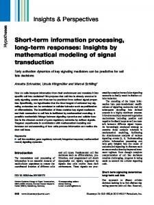
RESULTS Training 2 All the subjects learned the task, as can be seen from Figure 1, where the proportion of elements with the same base color is shown as a function of blocks of trials. The task is trivial when this proportion is 1.0, and impossible when it is .5. This proportion was automatically adjusted to keep accuracy around 75%–80%, which was maintained when approximately two thirds of the elements were of the same color. Experiment 1 Trials with response latencies greater than 4 sec were deleted from analysis, which reduced the database by less

Figure 1. The probability that stimulus elements will have the same base color, shown as a function of trials. The program adjusted this probability so that accuracy settled to around 78%.

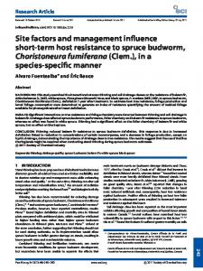
than 2%. Group A was somewhat more accurate than Group B (80% vs. 75%), but not significantly so [t(10) 5 1.52, p > .1]; the difference was due in part to Subject B6, whose accuracy was the lowest in this experiment (68%). The subjects made more errors when the foils occurred toward the end of a trial. The top panel of Figure 2 shows the probability of responding R (or G) when the element in the ith position was R (or G), respectively, for each of the subjects in Group A; the line runs through the average performance. The center panel contains the same information for Group B, and the bottom panel the average over all subjects. All the subjects except B6 (squares) were more greatly influenced by elements that occurred later in the list. Forgetting. Accuracy is less than perfect, and the control of the elements over the response varies as a function of their serial position. This may be because the information in the later elements blocks, or overwrites, that written by the earlier ones: retroactive interference. The average memory for a color depends on just how the influence of the elements changes as a function of their proximity to the end of the list, a change manifest in Figure 2. Suppose that each subsequent input decreases the memorial strength of a previous item by the factor q, as in the bulletin board example. This is an assumption of numerous models of short-term memory, including those of Estes (1950; Bower, 1994; Neimark & Estes, 1967), Heinemann (1983), and Roitblat (1983), and has been used as part of a model for visual information acquisition (Busey & Loftus, 1994). The last item will suffer no overwriting, the penultimate item an interference of q so that its weight will be 1 2 q, and so on. The influence of an element—its weight in memory—forms a geometrically decreasing series with parameter q and with the index i running from the end of the list to its beginning. The average value of the ith weight is wi 5

(1 2

q) i2 1.

(1)

Memory may also decay spontaneously: It has been shown in numerous matching-to-sample experiments that the accuracy of animals kept in the dark after the sample will decrease as the delay lengthens. Still, forgetting is usually greater when the chamber is illuminated during the retention interval or other stimuli are interposed (Grant, 1988; Shimp & Moffitt, 1977; cf. Kendrick, Tranberg, & Rilling, 1981; Wilkie, Summers, & Spetch, 1981). The mechanism of the recency effect may be due in part to the animals’ paying more attention to the cue as the trial nears its end, thus failing to encode the earliest elements. But these data make more sense looked back upon from the end of the trial where the curve is steepest, which is the vantage of the overwriting mechanism. All attentional models would look forward from the start of the interval and would predict more diffuse, uniform data with the passage of time. If, for instance, there was a constant probability of turning attention to the key over time, these influence curves would be a concave exponentialintegral, not the convex exponential that they seem to be.

WRITING TO MEMORY

21

this rule, performance would be perfect, and Figure 2 would show a horizontal line at the level of .67, the diagnosticity of any single element (see Appendix A). Designate the weight that each element has in the final decision as Wi , with i 5 1 designating the last item, i 5 2 the penultimate item, and so on. If, as assumed, the subjects attend only to green, the rule might be 12

Respond G if

å Wi S i > q , red otherwise. i =1

Figure 2. The probability that the response was G (or R) given that the element in the ith position was G (or R). The curves in the top panels run through the averages of the data; the curve in the bottom panel was drawn by Equations 1 and 2.

Deciding. The diagnosticity of each element is buffered by the 11 other elements in the list, so the effects shown in Figure 2 emerge only when data are averaged over many trials (here, approximately 2,000 per subject). It is therefore necessary to construct a model of the decision process. Assign the indices S i 5 0 and +1 to the color elements R and G, respectively. (In general, those indices may be given values of MR and MG , indicating the amount of memory available to such elements, but any particular values will be absorbed into the other parameters, and 0 and +1 are chosen for transparency.) One decision rule is to respond “G” when the sum of the color indices is greater than some threshold, theta (q, the criterion) and “R” otherwise. An appropriate criterion might be q 5 6, half-way between the number of green stimuli present on green-dominant trials (8) and the number present on red-dominant trials (4). If the pigeons followed

The indicated sum is the memory of green. Roberts and Grant (1974) have shown that pigeons can integrate the information in sample stimuli for at least 8 sec. If the weights were all equal to 1, the average sum on green-base trials would be 8, and subjects would be perfectly accurate. This does not happen. Not only are the weights less than 1, they are apparently unequal (Figure 2). What is the probability that a pigeon will respond G on a trial in which the ith stimulus is G? It is the probability that Wi plus the weighted sum of the other elements will carry the memory over the criterion. Both the elements, Si , and the weights, Wi , conceived as the probability of remembering the ith element, are random variables: Any particular stimulus element is either 0 or 1, with a mean on green-base trials of 2/3, a mean on redbase trials of 1/3, and an overall mean of 1/2. The animal will either remember that element (and thus add it to the sum) or not, with an average probability of remembering it being wi . The elements and weights are thus Bernoulli random variables, and the sum of their products over the 12 elements, Mi , forms a binomial distribution. With a large number of trials, it converges on a normal distribution. In Appendix B, the normal distribution is approximated by the logistic, and it is shown that the probability of a green response on trials in which the ith stimulus element is green and of a red response on trials in which the ith stimulus element is red is p( ; S i ) » (1 + e 2z )21,

(2)

with zi 5

[µ(N i ) 2 q )] . s

In this model, µ(Ni ) is the average memory of the dominant color given knowledge of the ith element and is a linear function of wi ( µ(Ni ) 5 awi + b; see Equation B13), q is the criterion above which such memories are called green, and below which they are called red, and s is proportional to the standard deviation, s 5 Ï3s /p. The scaling parameters involved in measuring µ(Ni ) may be absorbed by the other parameters of the logistic, to give (1 2 q) i21 2 q ¢ . s¢ The rate of memory loss is q: As q approaches 0, the influence curves become horizontal, and as it approaches 1, the influence of the last item grows toward exclusivzi 5

22

KILLEEN

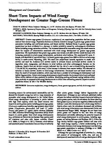
ity. The sum of the weights for an arbitrarily long sequence (i ® ¥) is 1 / q. This may be thought of as the total attentional/memorial capacity that is available for elements of this type—the size of the board relative to the size of the cards. Theta (q ) is the criterial evidence necessary for a green response. The variability of memory is s: The larger s is, the closer the influence curves will be to chance overall. The situation is symmetric for red elements. Equations 1 and 2 draw the curve through the average data in Figure 2, with q taking a value of .36, a value suggesting a memory capacity (1 / q) of about three elements. Individual subjects showed substantial differences in the values of q; these will be discussed below. As an alternative decision tactic, the pigeons might have subtracted the number of red elements remembered from the number of green and chosen green if the residue exceeded a criterion. This strategy is more efficient by a w , an advantage that may be outweighed by factor of Ï 2 its greater complexity. Because these alternative strategies are not distinguishable within the present experiments, the former, noncomparative strategy was assumed for simplicity in the experiments to be discussed below and in scenarios noted by Gaitan and Wixted (2000). Experiment 2 (ISI) In this experiment, the ISI was increased from 75 to 425 msec for the subjects in Group A. If the influence of each item decreases with the entry of the next item into memory, the serial-position curves should be invariant. If the influence decays with time, the apparent rate constants should increase by a factor of 1.7, since the trial duration has been increased from 6 to 10.2 sec, with 10.2/6 5 1.7. Results. The influence curve is shown in the top panel of Figure 3. The median value of q for these subjects was .40 in Experiment 1 and .37 here; the change in mean values was not significant [matched t(5) 5 0.19]. This lack of effect is even more evident in the bottom panel of Figure 3, where the influence curves for the two conditions are not visibly different. Discussion. This is not the first experiment to show an effect of intervening items— but not of intervening time— before recall. Norman (1966; Waugh & Norman, 1965) found that humans’ memory for items within lists of digits decreased geometrically, with no effect of ISI on the rate of forgetting (the average q for his visually presented lists was .28). Other experimenters have found decay during the ISI (e.g., Young, Wasserman, Hilfers, & Dalrymple, 1999). Roberts (1972b) found a linear decrease in percent correct as a function of ISIs ranging from 0 to 10 sec. He described a model similar to the present one, but in which decay was a function of time, not of intervening items. In a nice experimental dissociation of memory for number of flashes versus rate of flashing of keylights, Roberts, Macuda, and Brodbeck (1995) trained pigeons to discriminate long versus short stimuli and, in another condition, a large number of flashes from a small number (see Fig-

Figure 3. The probability that the response was G (or R) given that the element in the i th position was G (or R) in Experiment 2. The curve in the top panel runs through the average data; the curves in the bottom panel were drawn by Equations 1 and 2, with the filled symbols representing data from this experiment and the open symbols data from the same subjects in the baseline condition (Experiment 1).

ure 7 below). They concluded that in all cases, their subjects were counting the number of flashes, that their choices were based primarily on the most recent stimuli, and that the recency was time based rather than item based, because the relative impact of the final flashes increased with the interflash interval. Alsop and Honig (1991) came to a similar conclusion. The decrease in impact of early elements was attributed to a decrease in the apparent duration of the individual elements (Alsop & Honig, 1991) or in the number of counts representing them (Roberts et al., 1995), during the presentation of subsequent stimuli. The changes in the ISI were smaller in the present study and in Norman’s (1966: 0.1–1.0 sec) than in those evidencing temporal decay. When memory is tested after a delay, there is a decrease in performance even if the delay period is dark (although the decrease is greater in the light; Grant, 1988; Sherburne, Zentall, & Kaiser, 1998). It is likely that both overwriting and temporal decay are factors in forgetting, but with short ISIs the former are salient. McKone (1998) found that both factors affected repetition priming with words and nonwords, and Reitman (1974) found that both affected the forgetting of words when rehearsal was controlled. Wickelgren (1970) showed that both decay and interference affected memory of letters presented at different rates: Although

WRITING TO MEMORY forgetting was an exponential function of delay, rates of decay were faster for items presented at a higher rate. Wickelgren concluded that the decay depended on time but occurred at a higher rate during the presentation of an item. Wickelgren’s account is indistinguishable from ones in which there are dual sources of forgetting, temporal decay and event overwriting, with the balance naturally shifting toward overwriting as items are presented more rapidly. The passage of time is not just confounded with the changes in the environment that occur during it; it is constituted by those changes. Time is not a cause but a vehicle of causes. Claims for pure temporal decay are claims of ignorance concerning external inputs that retroactively interfered with memory. Such claims are quickly challenged by others who hypostasize intervening causes (e.g., Neath & Nairne, 1995). Attempts to block covert rewriting of the target item with competing tasks merely replace rewriting with overwriting (e.g., Levy & Jowaisas, 1971). The issue is not decay versus interference but, rather, the source and rate of interference; if these are occult and homogenous in time, time itself serves as a convenient avatar of them. Hereafter, decay will be used when time is the argument in equations and interference when identified stimuli are used as the argument, without implying that time is a cause in the former case or that no decrease in memory occurs absent those stimuli in the latter case. Experiment 3 (ITI) In this experiment, the ITI was increased to 30 sec for subjects in Group B. This manipulation halved the rate of reinforcement in real time and, in the process, devalued the background as a predictor of reinforcement. Will this enhance attention and thus accuracy? The subjects and apparatus were the same as those reported in Experiment 1 for Group B; the condition lasted for 20 sessions. Results. The longer ITI significantly improved performance, which increased from 75% to 79% [matched t(5) 5 4.6]. Figure 4 shows that this increase was primarily due to an improvement in overall performance, rather than to a differential effect on the slope of the influence curves. There was some steepening of the influence curves in this condition, but this change was not significant, although it approached significance with B6 removed from the analysis [matched t(4) 5 1.94, p >.05]. The curves through the average data in the bottom panel of Figure 4 share the same value of q 5 .33. Discussion. In the present experiment, the increased ITI improved performance and did so equally for the early and the late elements. It is likely that it did so both by enhancing attention and by insulating the stimuli (or responses) of the previous trial from those of the contemporary trial, thus providing increased protection from proactive interference. A similar increase in accuracy with increasing ITI has been repeatedly found in delayed matching-to-sample experiments (e.g., Roberts & Kraemer, 1982, 1984), as well as with traditional paradigms

23

Figure 4. The probability that the response was G (or R) given that the element in the ith position was G (or R) in Experiment 3. The curve in the top panel runs through the averages of the data; the curves in the bottom panel were drawn by Equations 1 and 2, with the filled symbols representing data from this experiment and the open symbols data from the same subjects in the baseline condition.

with humans (e.g., Cermak, 1970). Grant and Roberts (1973) found that the interfering effects of the f irst of two stimuli on judging the color of the second could be abated by inserting a delay between the stimuli; although they called the delay an ISI, it functioned as would an ITI to reduce proactive interference. APPLICATION, EXTENSION, AND DISCUSSIO N The present results involve differential stimulus summation: Pigeons were asked whether the sum of red stimulus elements was greater than the sum of green elements. In other summation paradigms—for instance, duration discrimination—they may be asked whether the sum of one type of stimulus exceeds a criterion (e.g., Loftus & McLean, 1999; Meck & Church, 1983). Counting is summation with multiple criteria corresponding to successive numbers (Davis & Pérusse, 1988; Killeen & Taylor, 2000). Effects analogous to those reported here have been discussed under the rubric response summation (e.g., Aydin & Pearce, 1997). The logistic/geometric provides a general model for summation studies: Equation 1 is a candidate model for discounting the events that are summed as a function of subsequent input, with Equation 2 capturing the decision process. This discussion begins by demonstrating the

24

KILLEEN

further utility of the logistic-geometric compound model for (1A) lists of varied stimuli with different patterns of presentation and (1B) repeated stimuli that are written to short-term memory and then overwritten during a retention interval. It then turns to (2) qualitative issues bearing on the interpretation of these data, (3) more detailed examination of the logistic shell and the related log-odds transformation, (4) the form of forgetting functions and their composition in a writing/overwriting model, and finally (5) the implications of averaging across different forgetting functions. Writing and Overwriting Heterogeneous Lists Young et al. (1999) trained pigeons to peck one screen location after the successive presentation of 16 identical icons and another after the presentation of 16 different icons, drawn from a pool of 24. After acquisition, they presented different patterns of similar and different icons: for instance, the first eight of one type, the second eight of a different type, four quartets of types, and so on. The various patterns are indicated on the x-axis in the top panel of Figure 5, and the resulting average proportions of different responses as bars above them. The compound model is engaged by assigning a value of +1 to a stimulus whenever it is presented for the first time on that list and of 2 1 when it is a repeat. Because we lack sufficient information to construct influence curves, the variable µ(Ni ) in Equation 2 is replaced with m S 5 åwi Si (see Appendix B), where m S is the average memory for novelty at the start of the recall interval: p » (1 + e 2 z) 2 1, z5

(3)

mS 2 q . } s

Equations 1 and 3, with parameters q 5 .1, q 5 2 .45, and s 5 .37, draw the curve of prediction above the bars. As w s / p. before, s 5 Ï 3 In Experiment 2a, the authors varied the number of different items in the list, with the variation coming either early in the list (dark bars) or late in the list. The overwriting model predicts that whatever comes last will have a larger effect, and the data show that this is generally the case. The predictions, shown in the middle panel of Figure 5, required parameters of q 5 .05, q 5 .06, and s 5 .46. In Experiment 2b, conducted on alternate days with 2a, Young et al. (1999) exposed the pigeons to lists of different lengths comprising items that were all the same or all different. List length was a strong controlling variable, with short lists much more difficult than long ones. This is predicted by the compound model only if the pigeons attend to both novelties and repetitions, instantiated in the model by adding (+1) to the cumulating evidence when a novelty is observed and subtracting from it (2 1) when a repetition is observed. So configured, the z-scores of short lists will be much closer to 0 than the z-scores of long lists. The data in the top two panels, where

Figure 5. The average proportion of different responses made by 8 pigeons when presented a series of 16 icons that were the same or different according to the patterns indicated in each panel (Young, Wasserman, Hilfers, & Dalrymple, 1999). The data are represented by the bars, and the predictions of the compound model (Equations 1 and 3) by the connected symbols.

list length was always 16, also used this construction but are equally well fit by assuming attention either to novelties alone or to repetitions alone (in which case the ignored events receive weights of 0). The data from Experiment 2b permit us to infer that the subjects do attend to both, since short strings with many novelties are more difficult than long strings with few novelties, even though

WRITING TO MEMORY both may have the same memorial strength for novelty (but different strengths for repetition). The predictions, shown in the bottom panel of Figure 5, used the same parameters as those employed in the analysis of Experiment 2a, shown above them. Delayed Recall Roberts et al. (1995) varied the number of flashes (F 5 2 or 8) while holding display time constant (S 5 4 sec) for one group of pigeons and, for another group, varied the display time (2 vs. 8 sec) while holding the number of flashes constant at 4. The animals were rewarded for judging which was greater (i.e., more frequent or of longer duration). Figure 6 shows their design for the stimuli. After training to criterion, they then tested memory for these stimuli at delays of up to 10 sec. The writing/overwriting model describes their results, assuming continuous forgetting through time with a rate constant of l 5 0.5/sec. Under this assumption, memory for items will increase as a cumulative exponential function of their display time (Loftus & McLean, 1999, provide a general model of stimulus input with a similar entailment). Since display time of the elements is constant, the (maximum) contribution of individual elements is set at 1. Their actual contribution to the memory of the stimulus at the start of the delay interval depends on their distance from it; in extended displays, the contribution from the first element has dissipated substantially by the start of the delay period (see, e.g., Figure 2). The cumulative contribution of the elements to memory at the start of the delay interval, m S , is n

mS = å e - l ti S i ,

(4)

i =1

where ti measure the time from the end of the ith flash until the start of the delay interval. This initial value of memory for the target stimulus will be larger on trials with the greater number of stimuli (the value of n is larger) or frequency of stimuli (the values of t are smaller).

25

During the delay, memories continue to decay exponentially, and when the animals are queried, the memory traces will be tested against a fixed criterion. This aggregation and exponential decay of memorial strength was also assumed by Keen and Machado (1999; also see Roberts, 1972b) in a very similar model, although they did not have the elements begin to decay until the end of the presentation epoch. Whereas their data were indifferent to that choice, both consistency of mechanism and the data of Roberts and associates recommend the present version, in which decay is is the same during both acquisition and retention. The memory for the stimulus at various delays d j is x j = mS e

- l dj

;

(5)

if this exceeds a criterion q, the animal indicates “greater.” Equation 3 may be used to predict the probability of responding “greater” given the greater (viz., longer/more numerous) stimulus. It is instantiated here as a logistic function of the distance of xj above threshold: Equation 3, with m S being the cumulation for the greater stimulus and zj 5

xj 2 q . } s

(6G)

The probability of responding “lesser” given the smaller stimulus is then a logistic function of the distance of xj below threshold: Equation 3, with mS being the cumulation for the lesser stimulus and zj 5

q 2 xj . } s

(6L)

To the extent memory decay continues through the interval, memory of the greater decays toward criterion, whereas memory of the lesser decays away from criterion, giving the latter a relative advantage. This provides a mechanism for the well-known choose-short effect (Spetch & Wilkie, 1983). It echoes an earlier model of accumulation and dissipation of memory offered by Roberts and Grant (1974) and is consistent with the data

Figure 6. The design of stimuli in the Roberts, Macuda, and Brodbeck (1995) experiment. On the right are listed the hypothetical memory strengths for number of flashes at the start of recall, as calculated from Equations 3–6.

26

KILLEEN ments). These were intrinsically easier/more accurate not only because they were helped by forgetting during the delay interval, but also because they were helped by inattention during the stimulus, and this is what the differences in s reflect. If the model is accurate, it should predict the one remaining free parameter, the level of memory at the beginning of the delay interval, mS. It does this by using the obtained value of l , 0.5/sec, in Equation 4. The bottom panel of Figure 7 shows that it succeeds in predicting the values of these parameters a priori, accounting for over 98% of their variance. (The nonzero intercept is a consequence of the choice of an arbitrary criterion q 5 1.) This ability to use a coherent model for both the storage (writing) and the report delay (overwriting) stages increases the degrees of freedom predicted without increasing the number used in constructing the mechanism, the primary advantage of hypothetical constructs such as short-term memory.

Figure 7. The decrease in memory for number of flashes as a function of delay interval in two conditions (Roberts, Macuda, & Broadbeck, 1995). Such decay aids judgments of “fewer flashes” that mediated these choices, as is shown by their uniformly high accuracy. The curves are from Equations 3–6. The bottom panel shows the hypothetical memory for number at the beginning of the delay interval as predicted by the summation model (Equation 4; abcissae) and as implied by the compound model (Equations 3, 5, and 6; ordinates).

of Roberts et al. (1995), as shown by Figure 7. In fitting these curves, the rate of memory decay ( l in Equation 5) was set to 0.5/sec. The value of the criterion was fixed at q 5 1 for all conditions, and mS was a free parameter. Judgments corresponding to the circles in Figure 7 required a value of 0.6 for s in both conditions, whereas values corresponding to the squares required a value of 1.1 for s in both conditions. The smaller measures of dispersion are associated with the judgments that were aided if the animal was inattentive on a trial (the “fewer flashes” judg-

Trial Spacing Effects Primacy versus recency. In the present experiments, there was no evidence of a primacy effect, in which the earliest items are recalled better than the intermediate items. Recency effects, such as those apparent in Figures 2– 4, are almost universally found, whereas primacy effects are less common (Gaffan, 1992). Wright (1998, 1999; Wright & Rivera, 1997) has identified conditions that foster primacy effects (well-practiced lists containing unique items, delay between review and report that differentially affects visual and auditory list memories, etc.), conditions absent from the present study. Machado and Cevik (1997) found primacy effects when they made it impossible for pigeons to discriminate the relative frequency of stimuli on the basis of their most recent occurrences and attributed such primacy to enhanced salience of the earliest stimuli. Presence at the start of a list is one way of enhancing salience; others include physically emphasizing the stimulus (Shimp, 1976) or the response (Lieberman, Davidson, & Thomas, 1985); such marking also improves coupling to the reinforcer and, thus, learning in traditional learning (Reed, Chih-Ta, Aggleton, & Rawlins, 1991; Williams, 1991, 1999) and memory (Archer & Margolin, 1970) paradigms. In the present experiment, there was massive proactive interference from prior lists, which eliminated any potential primacy effects (Grant, 1975). The improvement conferred by increasing the ITI was not differential for the first few items in the list. Generalization of the present overwriting model for primacy effects is therefore not assayed in this paper. Proactive Interference Stimuli presented before the to-be-remembered items may bias the subjects by preloading memory; this is called proactive interference. If the stimuli are random with respect to the current stimulus, such interference should eliminate any gains from primacy. Spetch and Sinha

WRITING TO MEMORY (1989; also see Kraemer & Roper, 1992) showed that a priming presentation of the to-be-remembered stimuli before a short stimulus impaired accuracy, whereas presentation before a long stimulus improved accuracy: Prior stimuli apparently summated with those to be remembered. Hampton, Shettleworth, and Westwood (1998) found that the amount of proactive interference varied with species and with whether or not observation of the to-be-remembered item was reinforced. Consummation of the reinforcer can itself fill memory, displacing prior stimuli and reducing interference. It can also block the memory of which response led to reinforcement (Killeen & Smith, 1984), reducing the effectiveness of frequent or extended reinforcement (Bizo, Kettle, & Killeen, 2001). These various effects are all consistent with the overwriting model, recognizing that the stimuli subjects are writing to memory may not be the ones the experimenter intended (Goldinger, 1996). Spetch (1987) trained pigeons to judge long/short samples at a constant 10-sec delay and then tested at a variety of delays. For delays longer than 10 sec, she found the usual bias for the short stimulus—the choose-short effect. At delays shorter than 10 sec, however, the pigeons tended to call the short stimulus “long.” This is consistent with the overwriting model: Training under a 10sec delay sets a criterion for reporting “long” stimuli quite low, owing to memory’s dissipation after 10 sec. When tested after brief delays, the memory for the short stimulus is much stronger than that modest criterion. In asymmetric judgments, such as present/absent, many/ few, long/short, passage of time or the events it contains will decrease the memory for the greater stimulus but is unlikely to increase the memory for the lesser stimulus, thus confounding the forgetting process with an apparent shift in bias. But the resulting performance reflects not so much a shift in bias (criterion) as a shift in memories of the greater stimulus toward the criterion and of the lesser one away from the criterion. If stimuli can be recoded onto a symmetric or unrelated set of memorial tags, this “bias” should be eliminated. In elegant studies, Grant and Spetch (1993a, 1993b) showed just this result: The choose-short effect is eliminated when other, nonanalogical codes are made available to the subjects and when differential reinforcement encourages the use of such codes (Kelly, Spetch, & Grant, 1999). As a trace cumulation/decumulation model of memory, the present theory shares the strengths and weaknesses of Staddon and Higa’s (1999a, 1999b) account of the choose-short effect. In particular, when the retention interval is signaled by a different stimulus than the ITI, the effect is largely abolished, with the probability of choosing short decreasing at about the same rate as that of choosing long (Zentall, 1999). These results would be consistent with trace theories if pigeons used decaying traces of the chamber illumination (rather than sample keylight) as the cue for their choices. Experimental tests of that rescue are lacking. Wixted and associates (Dougherty & Wixted, 1996; Wixted, 1993) analyze the choose-short effect as a kind

27

of presence/absence discrimination in which subjects respond on the basis of the evidence remembered and the evidence is a continuum of how much the stimuli seemed like a signal, with empty trials generally scoring lower than signal trials. Although some of their machinery is different (e.g., they assume that distributions of “present” and “absent” get more similar, rather than both decaying toward zero), many of their conclusions are similar to those presented here. Context These analyses focus on the number of events (or the time) that intervenes between a particular stimulus and the opportunity to report, but other factors are equally important. Roberts and Kraemer (1982) were among the first to emphasize the role of the ITI in modulating the level of performance, as was also seen in Experiment 3. Santiago and Wright (1984) vividly demonstrated how contextual effects change not only the level, but also the shape, of the serial position function. Impressive differences in level of forgetting occur depending on whether the delay is constant or is embedded in a set of different delays (White & Bunnell-McKenzie, 1985), or is similar to or different from the stimulus conditions during the ITI (Sherburne et al., 1998). Some of these effects might be attributed to changes in the quality of original encoding (affecting initial memorial strength, m S, relative to the level of variability, s); examples are manipulations of attention by varying the duration (Roberts & Grant, 1974), observation (Urcuioli, 1985; Wilkie, 1983), marking (Archer & Margolin, 1970), and surprisingness (Maki, 1979) of the sample. Other effects will require other explanatory mechanisms, including the different kinds of encoding (Grant, Spetch, & Kelly, 1997; Riley, Cook, & Lamb, 1981; Santi, Bridson, & Ducharme, 1993; Shimp & Moffitt, 1977). The compound model may be of use in understanding some of this panoply of effects; to make it so requires the following elaboration. THE COMPOUND MODEL The Logistic Shell The present model posits exponential changes in memorial strength, not exponential changes in the probability of a correct response. Memorial strength is not well captured by the unit interval on which probability resides. Two items with very different memorial strengths may still have a probability of recognition or recall arbitrarily close to 1.0: Probability is not an interval scale of strength. The logistic shell, and the logit transformation that is an intrinsic part of it, constitute a step toward such a scale (Luce, 1959). The compound model is a logistic shell around a forgetting function; its associated log-odds transform provides a candidate measure of memorial strength that is consistent with several intuitions, as will be outlined below. The theory developed here may be applied to both recognition and recall experiments. Recall failure may be due either to decay of target stimulus traces or to lack of

28

KILLEEN

associated cues (handles) sufficient to access those traces (see, e.g., Tulving & Madigan, 1970). By handle is meant any cue, conception, or context that restricts the search space; this may be a prime, a category name, the first letter of the word, or a physical location associated with the target, either provided extrinsically or recovered through an intrinsic search strategy. The handles are provided by the experimenter in cued recall and by the subject in free recall; in recognition experiments, the target stimulus is provided, requiring the subject to recall a stimulus that would otherwise serve as a handle (a name, presence or absence in training list, etc.). Handles may decay in a manner similar to target stimuli (Tulving & Psotka, 1972). The compound model is viable for cued recall, recognition, and free recall, with the forgetting functions in those paradigms being conditional on recovery of target stimulus, handle, or both, respectively. This treatment is revisited in the section on episodic theory, below. Paths to the Logit Ad hoc. If the probability p of an outcome is .80, in the course of 100 samples we expect to observe, on the average, 80 favorable outcomes. The odds for such an outcome are 80/20 5 p / (1 2 p) 5 4/1, and the odds against it are 1/4. The “odds” transformation maps probability from the symmetric unit interval to the positive continuum. Odds are intrinsically skewed: 4/1 is farther from indifference (1/1) than is 1/4, even though the distinction between favorable and unfavorable may signify an arbitrary assignment of 0 or 1, heads or tails, to an event. The log-odds transformation carries probability from the unit interval through the positive continuum of odds to the whole continuum, providing a symmetric map for probabilities centered at 0 when p is .50: æ p ö L b [ p] = log b ç 0 < p 0

(16)

Here, the rate of decay slows with time, as l / t. This differential entails a power law decay of memory, M t 5 M1t 2 l, which is sometimes found (e.g., Wixted & Ebbesen, 1997). The constant of integration, M1, corresponds to memory at t 5 1. Equations 13 and 16 are instances of the more general chemical rate equation: dM } 5 dt

2 l M g.

(17)

The rate equation (1) reduces to Equation 13 when g 5 1, (2) entails a power law decay, as does Equation 16, when g > 1, and (3) has memory grow with time, as might occur with consolidation, when g < 1. In their review of five models of perceptual memory, Laming and Scheiwiller (1985) answered their rhetorical

33

question, “What is the shape of the forgetting function,” with the admission, “Frankly, we do not know.” All of the models they studied, which included the exponential, accounted for the data within the limits of experimental error. The form of forgetting functions is likely to vary with the particular dependent variable used (Bogartz, 1990; Loftus & Bamber, 1990; Wixted, 1990; but see Wixted & Ebbesen, 1991). Since probabilities are bound by the unit interval and latencies are not, a function that fit one would require a nonlinear transformation to map it onto the other. Absent a strong theory that identifies the proper variables and their scale, the shape of this function is an illposed question (Wickens, 1998). Summary Both the variables responsible for increasing failure of recall as a function of time and the nature of the function itself are in contention. This is due, in part, to the use of different kinds of measurement in experimental reports. Here, two potential recall functions have been described: exponential and power functions, along with their differential equations and a general rate equation that takes them as special cases. If successful performance involves retention of multiple elements, each decaying according to one of these functions, the probability of recall failure as a function of time is given by their appropriate extreme value distributions. Most experiments involve both writing and overwriting; the exponential model was developed and applied to a representative experiment. Average Forms An important feature of the logit transformation of the dependent variable (Equations 7–10) is that, in linearizing the model, it preserves accurate representations over averages of subjects’ responses to stimuli that have different base detectability (m S) and chance (c) parameters. This recommends it as a dependent variable. But the logit does not preserve characteristics of the forgetting function if the parameter of f (t) itself varies. R. B. Anderson and Tweney (1997) raise only the latest voices in a chorus of cautions concerning the changes in the form of curves as a result of averaging—a concern that harks back to the controversy on the form of the “average” learning curve. Weitzman (1966) noted that “according to Bush and Mosteller (1955), statistical learning theorists ‘are forced to assume that all subjects have approximately the same parameter values’ in order to fit their models to real data. Despite its importance, however, psychologists have devoted little attention to this assumption” (p. 357). Recent exceptions are Van Zandt and Ratcliff’s (1995) elegant work on the “statistical mimicking” of one distribution by another owing to parameter variability, and Wickens’s (1998) fundamental analysis of the role of parameter variation in determining the form of forgetting functions. Consider some generalized measure of recall accuracy (r) involving a scaling factor (a), an intercept (b), and a function of time (or of interference occurring over time), f (t):

34

KILLEEN r 5 af (t) 1 b.

(18)

Equation 18 may represent the number of items recalled after different recall delays. If r 5 pcorrect , a » .5, and b 5 .5, it may represent the probability of being correct in a two-alternative forced-choice task in which the subject only guesses if recall fails; for a » 1 and b 5 0, it may represent that probability where chance level is zero. For r 5 precall , a 5 p / (1 2 g), and b 5 2g / (1 2 g), it is a correction of p correct for guessing. For r 5 L[ p t ], a 5 L[ p 0], and b 5 L[ p¥], it is Equation 9. If variability in r arises from Bernoulli processes with constant parameters, the best (unbiased, minimum variance) estimator of r at each point t ¢ through the forgetting process is simply the number of items correctly recalled (divided by the number of attempts, if r is a proportion). But if a, b, and l are random variables across subjects, across replications with a single subject, or across items, the average data will not conform to Equation 18 even though they were generated by it. In the simple case that the covariance of the random variables is zero, r 5 ag( l , t) 1 c,

(19)

with the overbar representing an arithmetic mean and g representing the average of the forgetting functions at time t. The average of the values that parameters a and c assumed while the data were being generated (Equation 18) are appropriate scaling and additive factors in the function representing the averaged data, Equation 19 (Appendix C). All that is needed to characterize the form of averaged data issuing from Equation 18 is g( l i , t). In the following, it is assumed that the form of the underlying function remains the same but its rate of decay varies from one sample to the next, whether these are samples of different attempts by the same person on the same item, by the same person on different items, or by different individuals. Exponential and Geometric Functions What is g(l i , t) for the exponential function f (t) 5 e2lt, over a range of values for the rate parameter l, if all we know is that the average value of lambda is l? That depends on the distribution of the particular values of rate constants in the experimental population. If we do not know this distribution, the assumption that is most general—a kind of worst-case or maximum-entropy assumption—is that the distribution of rate constants is itself exponential. This makes some intuitive sense, since we expect small rate constants to be more frequent than large ones: for instance, that lambda will be found in the interval 0–1 much more often than in the interval 100–101. Given a positive random variable about which we know only the mean, the exponential distribution entails the fewest other assumptions—that is, it is maximally random (Kagan, Linnick, & Rao, 1973; Skilling, 1989). Assume the frequency distribution of l in the population to be h(l) 5 l21e2l/l . Then, with f(l,t) 5 e2l t, integrating

over the entire range of possible decay rates 0–¥ provides the necessary weighted average: ¥

g (l , t ) = òl = h( l ) f ( l , t ) = 0

1 . lt +1

(20)

The average form is an inverse function of time that is sometimes called hyperbolic. An equivalent equation was used by McCarthy and Davison (1984) and Wixted (1989) to fit experimental data on delayed matching-to-sample experiments, by Mazur (1984) to predict the effect of delayed reinforcers on the traces of choice responses, and by Laming (1992) as a fundamental forgetting function for Brown– Peterson experiments. Alternate assumptions about the distribution of parameters give different average retention functions; Wickens (1998) provides a definitive review. In the case of interference-driven forgetting, the discrete analogue of the exponential is the geometric progression f(t) 5 (1 2 q) n. The max-ent distribution of a random variable on the unit interval is the uniform distribution. Averaged over the complete range of possible rate constants (q 5 0 to 1), the “null” hypothesis for the average forgetting function is g(t) 5

1 , n11

(21)

which is analogous to Equation 20. It is manifest that such hyperbolic functions may result from averaging exponential or geometric functions over a range of parameters. In the present experiment, the values of q were, in fact, uniformly distributed over the interval 0.0– 0.75—a straight line accounted for 95% of the variance in their values as a function of their rank order. This entails that the rate constant l will be exponentially distributed over a comparable range. The best estimate of the averaging function in this case is Equation21 with 0.25 n+1 subtracted from the numerator, reflecting a 6% faster decay for the first item than predicted by Equation 21, but no measurable difference thereafter. Power Decay Alternatively, assume f (t) 5 t 2l, t > 0, and invoke the entropy-maximizing function for l, h(l) 5 l21e2l/l . Averaging over this range, g(t) 5

1 . l ln(t) + 1

t > e2l/l

(22)

The average function is hyperbolic in the logarithm of time. Since it is convenient for f (0) 5 1, the offset power function f (t) 5 (t 1 1)2l is often used as a forgetting function. This changes the constraint to t ³ 0 but affects no other conclusions. Differentiation of the integrated term in Equations 20–22 returns the originating equation, as it must. If the upper and lower limits of integration converge, as would be the case if the rate constants were very tightly clustered (i.e., integrate between l¢ and l¢ + D, letting D ® 0), this

WRITING TO MEMORY is equivalent to the inverse operation, differentiation, and leaves us with the original functions. Therefore, this analysis shows that the proper model for averaged data will range from the originating equation when there is little variance in rate constants (small D) to its integrand (e.g., Equations 20–22) when there is substantial variation in rate constants. Analogous forms for acquisition are easily derived. Although the limits of integration here are arbitrary, they may be tailored to the particular context, either by estimating the values for extreme subjects or by treating the upper and lower limits in these equations as free parameters. In the latter case, for example, Equation 20 would become g( l, t) 5 (e 2 LLl t 2 e 2ULl t) / Dt, where D 5 l UL 2 l LL. In situations with little variability in forgetting rates, the estimated limits will be close (D ® 0), and the resulting curve will offer little advantage over the more parsimonious originating equation. This analysis assumes a flat distribution of rate constants between the limits of integration; more leptokurtic distributions will lie closer to the originating equations for the same range of parameters. Notice the family resemblance of Equations 20–22, with average strength decreasing as a hyperbolic function of time (or the input it carries) in the former two cases and of the logarithm of time in the last. As with the originating equations, the power model has memories decreasing more slowly with time than does the exponential. Wixted and Ebbesen (1997) found that power functions described both individual and averaged memory functions. Their subjects’ decay parameters were relatively tightly clustered, with semi-interquartile ranges of 0.07–0.17 in one condition and 0.10–0.17 in the other. With these limits of integration, Equation 22 is not discriminable from its originating power function. Note that this twofold range of the decay rates will leverage into substantial differences in recall over extended retention intervals; this shows that the originating equations may be robust over the averaging of what appear to be substantially different decay rates. Geometric/Binomial Model Finally, consider the major model of this analysis, Equation 3. No closed form solutions are available for integrating it over variations in the rate constant, but by converting to logits, Equation 20 is directly applicable. Figure 10 shows the results: In all cases, the averaging model accounts for more of the variance in the averaged data than does the originating logistic/geometric model. Data for individual subjects were, however, always better fit by the logistic/geometric model. The success of Equations 20 and 22 is therefore due to their ability to capture the effects of averaging, rather than to their being a better or more flexible model of the individual’s memorial process. Rubin and Wenzel (1996) In a survey of hundreds of experiments, Rubin and Wenzel (1996) found that, of two-parameter functions they studied, the generally best-fitting were the logarithmic [ y 5 k 2 l ln(t)], the exponential-root [ y 5 ke2 lÏ tw ], the

35

Figure 10. The logistic transformation (Equation 7) of the average influence functions collected in these experiments. The curves derive from Equations 19 and 20.

hyperbolic root [ y 5 1 / (k 1 lÏ wt )], and the power [ y 5 kt 2 l]. The above analysis shows that if the underlying functions f (t) are exponential or power functions, the averaged data will be linear transforms of Equations 20 or 22, respectively. Figure 11 shows average “data” generated by these functions as circles and the two best-fitting of Rubin and Wenzel’s functions drawn through them. The data in the top panel were generated by Equation 20, based on an underlying exponential decay of memory and the curves from best-fitting, hyperbolic-root (w 2 5 .98) and logarithmic (w 2 5 .95) functions. The exponential-root also accounted for 95% of the data variance. The data in the bottom panel were generated by Equation 22, based on an underlying power decay of memory and the best-fitting logarithmic (w 2 5 .96), and hyperbolicroot (w 2 5 .95) functions. The box scores for these empirical curve-fits will vary as a function of arbitrary considerations, such as how great a range is allowed for t and the distribution of the

36

KILLEEN over time. But averaging obscures our ability to understand the particulars of change in individual cases. A response scored correct (1) or incorrect (0) will generate traces from one trial to the next that are horizontal lines at one of those two levels. Averaging may convert the traces into exponentially decreasing functions, even though that graded process does not represent accuracy at any point in time on any trial. Nonetheless, such averaging over discontinuous processes is often optimal: A coin is never half of a head, yet the probability of a head may be precisely one half. In like manner, Equations 20–22 (or their instantiations for appropriate ranges of l) should not be dismissed as fixes for artifacts because they do not represent the state of events on any trial. They are characterizations sui generis, viable models for aggregating over a more abstract level of data—in particular, for averaging forgetting functions over a population of observers or items having different rates of decay.

Figure 11. The expected configuration of data averaged over a range of decay rates. The circles were located by Equations 19 and 20 (top panel, averaged exponential decay) and 19 and 22 (bottom panel, averaged power decay), with a 5 .75 and b 5 .25 in both cases. The curves are among those found by Rubin and Wenzel (1996) to provide a generally good fit to forgetting functions (see the text).

rate constants in the sample. The simple exponential function falls to an asymptote of 0 and would have been a contender if b had been set to 0 in the generating function. The important point is that averaging will warp the underlying forgetting functions into forms (Equations 20–22) that are consistent with Rubin and Wenzel’s (1996) meta-analysis. Intertemporal Choice These conclusions are not without implications for research on the control of behavior by anticipated outcomes—intertemporal choice (Ainslie, 1992). Researchers have generally assumed that the future is discounted according to an equation such as Equation 20 (e.g., Mazur, 1984)—or equivalently, that memory traces of choice responses are strengthened hyperbolically. It should now be clear that vicissitudes in the rate parameters of exponential discount functions could generate such hyperbolic forms. Levels of Analysis Averaging creates summary statistics that are more stable and representative than their constituents and thereby enhances our ability to visualize modal changes

Summary Laws describe the typical, and that is usually represented by the average. Just how and what to average entails a model of the process and the properties that one attempts to preserve under the averaging operation. Here, the probability of recall was represented as a Bernoulli process, and the resulting binomial distribution was approximated by the logistic distribution. The associated logit transformation faithfully represents the average initial and chance levels of recall by the parameters recovered from averaged data. The trajectory from initial to final recall— f(t)—is not preserved under the averaging operation. Instead, new curves result—g(l, t)—that are hyperbolic functions of time or of its logarithm but converge on the originating exponential or power functions as variance in rate parameters is reduced. Just as hyperbolic forgetting of past discriminative stimuli may be due to vicissitudes in rate parameters of exponential processes, hyperbolic discounting of future reinforcing stimuli may also arise from a similar morphing of exponential discount functions. SUMMARY AND CONCLUSIONS Memory for stimuli decreases both during their retention and during their recall (Guttenberger & Wasserman, 1985). A compound model provides a good treatment of both forgetting functions (Figures 2–4) and acquisition functions (Figure 9). Small variations in the brief ISIs had no effect on accuracy in the present experiment (Figure 3), suggesting that forgetting is event based. However, decay may occur during longer ISIs at slower, but nonzero, rates (Wickelgren, 1970), not discriminable from zero in this study. Longer ITIs facilitated recall (Figure 4). Although a geometric/exponential forgetting function embedded in a logistic shell accounted for the data under consideration, other forgetting functions, such as power functions, would have done almost as well. The decision to treat memorial strength (Equation 1 or Equations 20–22) and judgment (Equation 3) as sep-

WRITING TO MEMORY arate modules of a compound theory adds flexibility without an excessive burden of parameters. It has precedent in other analyses of influence in sequential patterns (e.g., Richards & Zhu, 1995). It leads toward familiar models (the log-odds SDT models) that are robust over averaging across varying initial detectability and criterion parameters. It is consistent with such mechanisms as control by relative recency and with multielement models (Figure 8). It intrinsically permits predictions of both the mean and the variance in judgments, which should repay the investment in two stages. It is directly applicable to experiments in which both target items and competing items are concurrently written to memory. Forms were developed to predict data derived from averages over studies or subjects with different rates of forgetting. These equations are similar to ones that describe data from a range of experiments (Rubin & Wenzel, 1996; Figure 11) and provided a better fit to averaged data from the present experiment (Figure 10), but not to the data of individual subjects, which were better served by the compound model with geometric memory loss. REFERENCES Ainslie, G. (1992). Picoeconomics. New York: Cambridge University Press. Allerup, P., & Ebro, C. (1998). Comparing differences in accuracy across conditions or individuals: An argument for the use of log odds. Quarterly Journal of Experimental Psychology, 51A, 409-424. Alsop, B. (1991). Behavioral models of signal detection and detection models of choice. In M. L. Commons, J. A. Nevin, & M. C. Davison (Eds.), Signal detection: Mechanisms, models, and applications (pp. 39-55). Hillsdale, NJ: Erlbaum. Alsop, B., & Honig, W. K. (1991). Sequential discrimination and relative numerosity discriminations in pigeons. Journal of Experimental Psychology: Animal Behavior Processes, 17, 386-395. Anderson, J. R., & Schooler, L. J. (1991). Reflections of the environment in memory. Psychological Science, 2, 396-408. Anderson, M. C., Bjork, R. A., & Bjork, E. L. (1994). Remembering can cause forgetting: Retrieval dynamics in long-term memory. Journal of Experimental Psychology: Learning, Memory, & Cognition, 20, 1063-1087. Anderson, R. B., & Tweney, R. D. (1997). Artifactual power curves in forgetting. Memory & Cognition, 25, 724-730. Archer, B. U., & Margolin, R. R. (1970). Arousal effects in intentional recall and forgetting. Journal of Experimental Psychology, 86, 8-12. Aydin, A., & Pearce, J. M. (1997). Some determinants of response summation. Animal Learning & Behavior, 25, 108-121. Bahrick, H. P. (1965). The ebb of retention. Psychological Review, 72, 60-73. Bahrick, H. P., Bahrick, P. O., & Wittlinger, R. P. (1975). Fifty years of memory for names and faces: A cross-sectional approach. Journal of Experimental Psychology: General, 104, 54-75. Belisle, C., & Cresswell, J. (1997). The effects of a limited memory capacity on foraging behavior. Theoretical Population Biology, 52, 78-90. Bizo, L. A., Kettle, L. C., & Killeen, P. R. (2001). Rats don’t always respond faster for more food: The paradoxical incentive effect. Animal Learning & Behavior, 29, 66-78. Bogartz, R. S. (1990). Evaluating forgetting curves psychologically. Journal of Experimental Psychology: Learning, Memory, & Cognition, 16, 138-148. Bower, G. H. (1994). A turning point in mathematical learning theory. Psychological Review, 101, 290-300. Bower, G. H., Thompson-Schill, S., & Tulving, E. (1994). Reduc-

37

ing retroactive interference: An interference analysis. Journal of Experimental Psychology: Learning, Memory, & Cognition, 20, 51-66. Busey, T. A., & Loftus, G. R. (1994). Sensory and cognitive components of visual information acquisition. Psychological Review, 101, 446-469. Cermak, L. S. (1970). Decay of interference as a function of the intertrial interval in short-term memory. Journal of Experimental Psychology, 84, 499-501. Couvillon, P. A., Arincorayan, N. M., & Bitterman, M. E. (1998). Control of performance by short-term memory in honeybees. Animal Learning & Behavior, 26, 469-474. Daniel, T. C., & Ellis, H. C. (1972). Stimulus codability and longterm recognition memory for visual form. Journal of Experimental Psychology, 93, 83-89. Davis, H., & Pérusse, R. (1988). Numerical competence in animals. Behavioral & Brain Sciences, 11, 561-579. Davison, M., & Nevin, J. A. (1999). Stimuli, reinforcers and behavior: An integration. Journal of the Experimental Analysis of Behavior, 71, 439-482. Dittrich, W. H., & Lea, S. E. G. (1993). Motion as a natural category for pigeons: Generalization and a feature-positive effect. Journal of the Experimental Analysis of Behavior, 59, 115-129. Dougherty, D. H., & Wixted, J. T. (1996). Detecting a nonevent: Delayed presence-versus-absence discrimination in pigeons. Journal of the Experimental Analysis of Behavior, 65, 81-92. Estes, W. K. (1950). Toward a statistical theory of learning. Psychological Review, 57, 94-107. Estes, W. K. (1956). The problem of inference from curves based on group data. Psychological Bulletin, 53, 134-140. Evans, M., Hastings, N., & Peacock, B. (1993). Statistical distributions (2nd ed.). New York: Wiley. Gaffan, E. A. (1992). Primacy, recency, and the variability of data in studies of animals’ working memory. Animal Learning & Behavior, 20, 240-252. Gaitan, S. C., & Wixted, J. T. (2000). The role of “nothing” in memory for event duration in pigeons. Animal Learning & Behavior, 28, 147-161. Goldinger, S. D. (1996). Words and voices: Episodic traces in spoken word identification and recognition memory. Journal of Experimental Psychology: Learning, Memory, & Cognition, 22, 1166-1183. Goldinger, S. D. (1998). Echoes of echoes? An episodic theory of lexical access. Psychological Review, 105, 251-279. Grant, D. S. (1975). Proactive interference in pigeon short-term memory. Journal of Experimental Psychology: Animal Behavior Processes, 1, 207-220. Grant, D. S. (1988). Sources of visual interference in delayed matching-to-sample with pigeons. Journal of Experimental Psychology: Animal Behavior Processes, 14, 368-275. Grant, D. S., & Roberts, W. A. (1973). Trace interaction in pigeon short-term memory. Journal of Experimental Psychology, 101, 2129. Grant, D. S., & Spetch, M. L. (1993a). Analogical and nonanalogical coding of samples differing in duration in a choice-matching task in pigeons. Journal of Experimental Psychology: Animal Behavior Processes, 19, 15-25. Grant, D. S., & Spetch, M. L. (1993b). Memory for duration in pigeons: Dissociation of choose-short and temporal-summation effects. Animal Learning & Behavior, 21, 384-390. Grant, D. S., Spetch, M., & Kelly, R. (1997). Pigeons’ coding of event duration in delayed matching-to-sample. In C. Bradshaw & E. Szabadi (Eds.), Time and behaviour: Psychological and neurobehavioural analyses (Vol. 120, pp. 217-264). Amsterdam: Elsevier. Gronlund, S. D., & Elam, L. E. (1994). List-length effect: Recognition accuracy and variance of underlying distributions. Journal of Experimental Psychology: Learning, Memory, & Cognition, 20, 1355-1369. Gumbel, E. J. (1958). Statistics of extremes. New York: Columbia University Press. Guttenberger, V. T., & Wasserman, E. A. (1985). Effects of sample duration, retention interval, and passage of time in the test on pigeons’ matching-to-sample performance. Animal Learning & Behavior, 13, 121-128.

38

KILLEEN

Hampton, R. R., Shettleworth, S. J., & Westwood, R. P. (1998). Proactive interference, recency, and associative strength: Comparisons of black-capped chickadees and dark-eyed juncos. Animal Learning & Behavior, 26, 475-485. Harper, D. N., & White, K. G. (1997). Retroactive interference and rate of forgetting in delayed matching-to-sample performance. Animal Learning & Behavior, 25, 158-164. Hearst, E. (1991). Psychology and nothing. American Scientist, 79, 432-443. Heinemann, E. G. (1983). A memory model for decision processes in pigeons. In M. L. Commons, R. J. Herrnstein, & A. R. Wagner (Eds.), Quantitative analysis of behavior: Vol. 4. Discrimination processes (pp. 3-19). Cambridge, MA: Ballinger. Hintzman, D. L. (1986). “Schema abstraction” in a multiple-trace memory model. Psychological Review, 93, 411-428. Johnson, R. A., Rissing, S. W., & Killeen, P. R. (1994). Differential learning and memory by co-occurring ant species. Insectes Sociaux, 41, 165-177. Kagan, A. M., Linnick, Y. V., & Rao, C. R. (1973). Characterization problems in mathematical statistics. New York: Wiley. Keen, R., & Machado, A. (1999). How pigeons discriminate the relative frequency of events. Journal of the Experimental Analysis of Behavior, 72, 151-175. Kelly, R., Spetch, M. L., & Grant, D. S. (1999). Influence of nonmemorial factors on manifestation of short-sample biases in choice and successive matching-to-duration tasks with pigeons. Journal of Experimental Psychology: Animal Behavior Processes, 25, 297-307. Kendrick, D. F., Jr., Tranberg, D. K., & Rilling, M. (1981). The effects of illumination on the acquisition of delayed matching-to-sample. Animal Learning & Behavior, 9, 202-208. Killeen, P. R., & Smith, J. P. (1984). Perception of contingency in conditioning: Scalar timing, response bias, and the erasure of memory by reinforcement. Journal of Experimental Psychology: Animal Behavior Processes, 10, 333-345. Killeen, P. R., & Taylor, T. J. (2000). How the propagation of error through stochastic counters affects time discrimination and other psychophysical judgments. Psychological Review, 107, 430-459. Kraemer, P. J., & Golding, J. M. (1997). Adaptive forgetting in animals. Psychonomic Bulletin & Review, 4, 480-491. Kraemer, P. J., & Roper, K. L. (1992). Matching-to-sample performance by pigeons trained with visual-duration compound samples. Animal Learning & Behavior, 20, 33-40. Laming, D. (1992). Analysis of short-term retention: Models for Brown– Peterson experiments. Journal of Experimental Psychology: Learning, Memory, & Cognition, 18, 1342-1365. Laming, D., & Scheiwiller, P. (1985). Retention in perceptual memory: A review of models and data. Perception & Psychophysics, 37, 189-197. Langley, C. M. (1996). Search images: Selective attention to specific visual features of prey. Journal of Experimental Psychology: Animal Behavior Processes, 22, 152-163. Levy, C. M., & Jowaisas, D. (1971). Short-term memory: Storage interference or storage decay? Journal of Experimental Psychology, 88, 189-195. Lieberman, D. A., Davidson, F. H., & Thomas, G. V. (1985). Marking in pigeons: The role of memory in delayed reinforcement. Journal of Experimental Psychology: Animal Behavior Processes, 11, 611-624. Link, S. W. (1992). The wave theory of difference and similarity. Hillsdale, NJ: Erlbaum. Loftus, G. R. (1985). Evaluating forgetting curves. Journal of Experimental Psychology: Learning, Memory, & Cognition, 11, 397-406. Loftus, G. R., & Bamber, D. (1990). Learning–forgetting independence, unidimensional memory models, and feature models: Comment on Bogartz (1990). Journal of Experimental Psychology: Learning, Memory, & Cognition, 16, 916-926. Loftus, G. R., & McLean, J. E. (1999). A front end to a theory of picture recognition. Psychonomic Bulletin & Review, 6, 394-411. Luce, R. D. (1959). Individual choice behavior. New York: Wiley. Machado, A., & Cevik, M. (1997). The discrimination of relative frequency by pigeons. Journal of the Experimental Analysis of Behavior, 67, 11-41. Maki, W. S. (1979). Pigeons’ short-term memories for surprising vs. ex-

pected reinforcement and nonreinforcement. Animal Learning & Behavior, 7, 31-37. Mazur, J. E. (1984). Tests of an equivalence rule for fixed and variable delays. Journal of Experimental Psychology: Animal Behavior Processes, 10, 426-436. McCarthy, D., & Davison, M. (1984). Delayed reinforcement and delayed choice in symbolic matching to sample: Effects on stimulus discriminability. Journal of the Experimental Analysis of Behavior, 46, 293-303. McCarthy, D., & White, K. G. (1987). Behavioral models of delayed detection and their application to the study of memory. In M. L. Commons, J. E. Mazur, J. A. Nevin, & H. Rachlin (Eds.), Quantitative analysis of behavior: Vol. 5. The effect of delay and intervening events on reinforcement value (pp. 29-54). Hillsdale, NJ: Erlbaum. McKone, E. (1998). The decay of short-term implicit memory: Unpacking lag. Memory & Cognition, 26, 1173-1186. Meck, W. H., & Church, R. M. (1983). A mode control model of counting and timing processes. Journal of Experimental Psychology: Animal Behavior Processes, 9, 320-334. Neath, I., & Nairne, J. S. (1995). Word-length effects in immediate memory: Overwriting trace decay theory. Psychonomic Bulletin & Review, 2, 429-441. Neimark, E. D., & Estes, W. K. (1967). Stimulus sampling theory. San Francisco: Holden-Day. Norman, D. A. (1966). Acquisition and retention in short-term memory. Journal of Experimental Psychology, 72, 369-381. Plaisted, K. C., & Mackintosh, N. J. (1995). Visual-search for cryptic stimuli in pigeons: Implications for the search image and search rate hypotheses. Animal Behaviour, 50, 1219-1232. Rasch, G. (1960). Probabilistic models for some intelligence and attainment tests. Copenhagen: Danmarks Pædagogiske Institut. Ratcliff, R., Clark, S. E., & Shiffrin, R. M. (1990). The list-strength effect: I. Data and discussion. Journal of Experimental Psychology: Learning, Memory, & Cognition, 16, 163-178. Ratcliff, R., McKoon, G., & Tindall, M. (1994). Empirical generality of data from recognition memory receiver-operating characteristic functions and implications for the global memory models. Journal of Experimental Psychology: Learning, Memory, & Cognition, 20, 763-785. Reed, P., Chih-Ta, T., Aggleton, J. P., & Rawlins, J. N. P. (1991). Primacy, recency, and the von Restorff effect in rats’ nonspatial recognition memory. Journal of Experimental Psychology: Animal Behavior Processes, 17, 36-44. Reitman, J. S. (1974). Without surreptitious rehearsal, information in short-term memory decays. Journal of Verbal Learning & Verbal Behavior, 13, 365-377. Riccio, D. C., Rabinowitz, V. C., & Axelrod, S. (1994). Memory: When less is more. American Psychologist, 49, 917-926. Richards, V. M., & Zhu, S. (1995). Relative estimates of combination weights, decision criteria, and internal noise based on correlation coefficients. Journal of the Acoustical Society of America, 95, 423-434. Riley, D. A., Cook, R. G., & Lamb, M. R. (1981). A classification and analysis of short-term retention codes in pigeons. In G. H. Bower (Ed.), The psychology of learning and motivation (Vol. 15, pp. 5179). New York: Academic Press. Roberts, W. A. (1972a). Free recall of word lists varying in length and rate of presentation: A test of total-time hypotheses. Journal of Experimental Psychology, 92, 365-372. Roberts, W. A. (1972b). Short-term memory in the pigeon: Effects of repetition and spacing. Journal of Experimental Psychology, 94, 74-83. Roberts, W. A., & Grant, D. S. (1974). Short-term memory in the pigeon with presentation time precisely controlled. Learning & Motivation, 5, 393-408. Roberts, W. A., & Kraemer, P. J. (1982). Some observations of the effects of intertrial interval and delay on delayed matching to sample in pigeons. Journal of Experimental Psychology: Animal Behavior Processes, 8, 342-353. Roberts, W. A., & Kraemer, P. J. (1984). Temporal variables in delayed matching to sample. In J. Gibbon & L. Allan (Eds.), Timing and time perception (Annals of the New York Academy of Sciences, Vol. 423, pp. 335-345). New York: New York Academy of Sciences.

WRITING TO MEMORY Roberts, W. A., Macuda, T., & Brodbeck, D. R. (1995). Memory for number of light flashes in the pigeon. Animal Learning & Behavior, 23, 182-188. Roitblat, H. L. (1983). Pigeon working memory: Models for delayed matching-to-sample. In M. L. Commons, R. J. Herrnstein, & A. R. Wagner (Eds.), Quantitative analysis of behavior: Vol. 4. Discrimination processes (pp. 161-181). Cambridge, MA: Ballinger. Rubin, D. C., & Wenzel, A. E. (1996). One hundred years of forgetting: A quantitative description of retention. Psychological Review, 103, 734-760. Sadralodabai, T., & Sorkin, R. D. (1999). Effect of temporal position, proportional variance, and proportional duration on decision weights in temporal pattern discrimination. Journal of the Acoustical Society of America, 105, 358-365. Santi, A., Bridson, S., & Ducharme, M. J. (1993). Memory codes for temporal and nontemporal samples in many-to-one matching by pigeons. Animal Learning & Behavior, 21, 120-130. Santiago, H. C., & Wright, A. A. (1984). Pigeon memory: Same/ different concept learning, serial probe recognition acquisition, and probe delay effects on the serial position function. Journal of Experimental Psychology: Animal Behavior Processes, 10, 498-512. Sherburne, L. M., Zentall, T. R., & Kaiser, D. H. (1998). Timing in pigeons: The choose-short effect may result from pigeons’ “confusion” between delay and intertrial intervals. Psychonomic Bulletin & Review, 5, 516-522. Shimp, C. P. (1976). Short-term memory in the pigeon: Relative recency. Journal of the Experimental Analysis of Behavior, 25, 55-61. Shimp, C. P., & Moffitt, M. (1977). Short-term memory in the pigeon: Delayed-pair-comparison procedures and some results. Journal of the Experimental Analysis of Behavior, 28, 13-25. Skilling, J. (1989). Maximum entropy and Bayesian methods. Dordrecht: Kluwer. Spear, N. E. (1978). The processing of memories: Forgetting and retention. Hilladale, NJ: Erlbaum. Spetch, M. L. (1987). Systematic errors in pigeons’ memory for event duration: Interaction between training and test delay. Animal Learning & Behavior, 15, 1-5. Spetch, M. L., & Sinha, S. S. (1989). Proactive effects in pigeons’ memory for event durations: Evidence for analogical retention. Journal of Experimental Psychology: Animal Behavior Processes, 15, 347-357. Spetch, M. L., & Wilkie, D. M. (1983). Subjective shortening: A model of pigeons’ memory for event duration. Journal of Experimental Psychology: Animal Behavior Processes, 9, 14-30. Staddon, J. E. R., & Higa, J. J. (1999a). The choose-short effect and trace models of timing. Journal of the Experimental Analysis of Behavior, 72, 473-478. Staddon, J. E. R., & Higa, J. J. (1999b). Time and memory: Towards a pacemaker-free theory of interval timing. Journal of the Experimental Analysis of Behavior, 71, 215-251. Sveshnikov, A. A. (1978). Problems in probability theory, mathematical statistics and theory of random functions (Scripta Technica, Inc., Trans.). New York: Dover. (Original work published 1968) Tulving, E., & Madigan, S. A. (1970). Memory and verbal learning. Annual Review of Psychology, 21, 437-484. Tulving, E., & Psotka, J. (1972). Retroactive inhibition in free recall: Inaccessibility of information available in the memory store. Journal of Experimental Psychology, 87, 1-8. Urcuioli, P. (1985). On the role of differential sample behaviors in matching to sample. Journal of Experimental Psychology: Animal Behavior Processes, 11, 502-519. Van Zandt, T., & Ratcliff, R. (1995). Statistical mimicking of reaction

39

time data: Single-process models, parameter variability, and mixtures. Psychonomic Bulletin & Review, 2, 20-54. Vaughan, W., Jr. (1984). Pigeon visual memory capacity. Journal of Experimental Psychology: Animal Behavior Processes, 10, 256-271. Waugh, N. C., & Norman, D. A. (1965). Primary memory. Psychological Review, 72, 89-104. Weitzman, R. A. (1966). Statistical learning models and individual differences. Psychological Review, 73, 357-364. White, K. G. (1985). Characteristics of forgetting functions in delayed matching to sample. Journal of the Experimental Analysis of Behavior, 44, 15-34. White, K. G., & Bunnell-McKenzie, J. (1985). Potentiation of delayed matching with variable delays. Animal Learning & Behavior, 13, 397-402. White, K. G., & Wixted, J. T. (1999). Psychophysics of remembering. Journal of the Experimental Analysis of Behavior, 71, 91-113. Wickelgren, W. A. (1970). Time, interference, and rate of presentation in short-term recognition memory for items. Journal of Mathematical Psychology, 7, 219-235. Wickens, T. D. (1998). On the form of the retention function: Comment on Rubin and Wenzel (1996): A quantitative description of retention. Psychological Review, 105, 379-386. Wilkie, D. M. (1983). Reinforcement for pecking the sample facilitates pigeons’ delayed matching to sample. Behaviour Analysis Letters, 3, 311-316. Wilkie, D. M., Summers, R. J., & Spetch, M. L. (1981). Effect of delay-interval stimuli on delayed symbolic matching to sample in the pigeon. Journal of the Experimental Analysis of Behavior, 35, 153-160. Williams, B. A. (1991). Marking and bridging versus conditioned reinforcement. Animal Learning & Behavior, 19, 264-269. Williams, B. A. (1999). Associative competition in operant conditioning: Blocking the response–reinforcer association. Psychonomic Bulletin & Review, 6, 618-623. Wixted, J. T. (1989). Nonhuman short-term memory: A quantitative analysis of selected findings. Journal of the Experimental Analysis of Behavior, 52, 409-426. Wixted, J. T. (1990). Analyzing the empirical course of forgetting. Journal of Experimental Psychology: Learning, Memory, & Cognition, 16, 927-935. Wixted, J. T. (1993). A signal detection analysis of memory for nonoccurrence in pigeons. Journal of Experimental Psychology: Animal Behavior Processes, 19, 400-411. Wixted, J. T., & Ebbesen, E. B. (1991). On the form of forgetting. Psychological Science, 2, 409-415. Wixted, J. T., & Ebbesen, E. B. (1997). Genuine power curves in forgetting: A quantitative analysis of individual subject forgetting functions. Memory & Cognition, 25, 731-739. Wright, A. A. (1998). Auditory list memory in rhesus monkeys. Psychological Science, 9, 91-98. Wright, A. A. (1999). Auditory list memory and interference processes in monkeys. Journal of Experimental Psychology: Animal Behavior Processes, 25, 284-296. Wright, A. A., & Rivera, J. J. (1997). Memory of auditory lists by rhesus monkeys (Macaca mulatta). Journal of Experimental Psychology: Animal Behavior Processes, 23, 441-449. Young, M. E., Wasserman, E. A., Hilfers, M. A., & Dalrymple, R. (1999). The pigeon’s variability discrimination with lists of successively presented stimuli. Journal of Experimental Psychology: Animal Behavior Processes, 25, 475-490. Zentall, T. R. (1999). Support for a theory of memory for event duration must distinguish between test-trial ambiguity and actual memory loss. Journal of the Experimental Analysis of Behavior, 72, 467-472.

(Continued on next page)

40

KILLEEN APPENDIX A Diagnosticity Given that a single element Si has color Cj (C0 5 red, C 1 5 green), what is the probability that Cj is also the base color SB for the trial? From Bayes theorem it is p{(SB 5 Cj ) | (Si 5 C j )} 5

p{(Si 5 C j ) | (SB 5 Cj )} 3 p(S B 5 Cj ) p(Si 5 Cj )

.

(A1)

The probability that a particular element has color Cj , given that that is the base on that trial, p{(Si 5 Cj ) | (SB 5 CJ )}, is 23. The prior probability that the base color will be C j on any trial, p(SB 5 Cj ), is 12. The base rate for an element to have color C j is also 12. Therefore Equation A1 resolves to p{(SB 5 Cj ) | (Si 5 Cj )} = 23. APPENDIX B Deciding Investigators sometimes apply an exponential function directly to recall data. Such curve-fitting implies that the controlling variable (memory) equals one particular dependent variable (viz., probability of recall) whose boundary conditions are the same as those of the exponential (viz., 1 and 0). But a new phone number might be immediately repeated with the same accuracy as a home phone number; yet in no wise would we ascribe equal memorial strength to them. A more general model is constructed here, one in which attrition occurs not to response probabilities, but to memories, whose strengths are transformed into response probability using a Thurstone model.

Unconditional Probability of a G Response

The base probability of responding G on a trial comprises the probabilities that the memory of green exceeds criterion on green- and red-base trials, which occur with equal probability. Consider the random variable MS , the number of green elements remembered at the end of a sample, where S j is 1 if the element is green and Wj is 1 if the element is remembered: 12

M S = å Wj S j .

(B1)

j

The expected value of MS , m S , is the sum of the product of the expectations of its factors: 12

m S = å wj m (S j ),

(B2)

j

where w j 5 µ(Wj ). The average value of S j on any trial is p (here, 13 on red-base trials, 23 on green-base trials, and overall 1/2). When wj is a geometric progression (Equation 1 in the text), the average memory of green at the end of the sample is mS 5 p

1 2 (1 2 q)12 . q

(B3)

In the limits, as q ® 1, only the last item is recalled, and mS ® p; and as q ® 0, all are recalled, and mS ® 12p. For q 5 .2, on green-base trials mS 5 3.10, on red-base trials mS 5 1.55, and on the average m S 5 2.33. Ignorant of which base trial is scheduled, subjects would do well to respond G whenever the memory of green on a trial exceeds 2.33 elements, and red otherwise. If they adopt this strategy, what is the probability of responding G—that is, what is the p( 5 1)? Because we are sampling repeatedly from populations of binary random variables and calculating the sums of those samples, the relevant densities of memory strengths are Bernoulli processes that approximate the normal. The variance, which is aggravated by encoding failure, lapse of attention, and so forth, is treated here as a free parameter, s 2 > 0. The central limit theorem permits us to write ¥

p ( = 1) » òq N [ x , m Ss ] dx.

(B4)

The logistic approximation to the normal is more convenient to evaluate and leads to a concise treatment of the decision process in terms of logits. The area under the integral in Equation B4 is approximately p( 5 1) » (1 + e 2z)21,

(B5)

with z 5 (mS 2 q) / s,

(B6)

WRITING TO MEMORY APPENDIX B (Continued) where, for the logistic, s 5 Ï 3w s / p . From the above example, mS is either 3.10 or 1.55, depending on the base of the trial. Theta (q ) is the criterion for deciding G or R; in the above example, an optimal value for it was 2.33. Under differential payoff, q may shift to maximize the expected value of the decisions. The logit transform of p is é p (R = 1) ù ln ê ú = z = ( mS - q ) / s. ë 1 - p (R = 1) û

(B7)

Influence Curves Equation B1 expands to éæ 12 ù éæ 12 ù ö ö p( = 1) = 1 p êç åWj S j ÷ > q | G is baseú + 1 p êç å Wj S j ÷ > q | R is baseú . 2 êëè j 2 ø ø úû êëè j úû The first bracket governs the green-base trials, during which the probability that Sj 5 1 is 2/3; the second bracket governs the red-base trials. This expansion opens the door for consideration of the probability of a G response, given knowledge of one of the elements. Consider the case in which the ith element is green, Si 5 1. Then, the probability of this being a green-base trial increases from 1/2 to 2/3 (see Appendix A), and 12 12 é ù é ù p( = 1 | Si = 1) = 2 p êWi + å Wj S j > q | G is base and S i = 1ú + 1 p êWi + å Wj S j > q | R is base and Si = 1ú . 3 ë 3 j j ¹i û ë û For conciseness,B1 write the number of green elements remembered at the end of green-base trials on which the ith element is known to be green as NG i , and the number remembered at the end of red-base trials on which the ith element is known to be green as NRi : 12

NGi = Wi + å Wj S j j ¹i

G is base and S i = 1

(B8)

R is base and S i = 1

(B9)

and 12

NRi = Wi + å Wj S j . j ¹i

Then, p( 5

1 | Si 5

1) 5

2 1 } p[NGi > q ] + } p[NRi > q ]. 3 3

(B10)

The probability of responding “green” given a green element is a weighted mixture of the base probabilities of responding “green” on green-base trials (the first bracket, corresponding to a hit, or true positive) and responding “green” on a red-base trial (the second bracket, corresponding to a false alarm, or false positive). The complements of these probabilities give, respectively, the probabilities of a false negative and of a true negative. The mean of these impressions of green, µ(NGi ) and µ(NR i ), equal the sum of the products of the random variables they comprise: 12

m( NGi ) = m(Wi ) + å m (Wj ) m( S j ),

(B11)

j¹i

with a symmetric expression for the mean on red-base trials. On green-base trials, the expected value of Sj is 8/12; having sampled one green stimulus, this becomes pG 5 7/11. On green-base trials, the expected value of S j is 4/12; having sampled one green stimulus, this becomes pR 5 3/11. Then, 12

m( NGi ) = m(Wi ) + pG å m (Wj ) j ¹i

12

= (1 - pG ) m (Wi ) + pG å m (Wi ). j =1

Notice that in the second line, the summation now extends over all stimuli. Assuming the geometric decrease in the weights posited by Equation 1 in the text, µ(W i ) 5 (1 2 q) i2 1, and the sum of the 12 weights is

41

42

KILLEEN APPENDIX B (Continued) 12

å = å m (Wj ) = j =1

1 - (1 - q )12 . q

Then,

m( NGi ) = (1 - pG )(1 - q )i-1 + pG å , and symmetrically for red-based trials,

m( NRi ) = (1 - pR )(1 - q )i-1 + pR å . Invoking the central limit theorem, we may now write Equation B10 as ¥ ¥ p( R = 1 | Si = 1) » 2 ò N [ x, m ( NGi )s ]dx + 1 ò N [ x, m ( NRi )s ]dx, 3 q 3 q

(B12)

with the first term representing the probability of true positives and the second that of false positives. In analyzing the influence curves in this experiment, these probabilities were combined. That mixture is approximately normal, with mean

[

] [

]

m( N i ) = 2 (1 - pG )(1 - q )i-1 + pG S + 1 (1 - pR )(1 - q )i-1 + pR S . 3 3

(B13)

For the parameters of the present experiments, this evaluates as

m( N i ) = 16 (1 - q)i-7 + 17 å , 33 33 and ¥

p( = 1 | Si = 1) » òq N [ x , m ( N i )s ]dx.

(B14)

By symmetry, a similar model governs the probability of saying “red” given a red element, with the integrals running from 2 ¥ to q . The logistic approximation to the normal that gives the area under the integral in Equation B14 is p( 5

1 | Si 5

1) » [1 1

e2

zi]2 1,

(B15)

with zi 5

[µ(Ni ) 2

q ] / s,

and s 5 Ï 3w s / p. This is the result given in the text. The influence curves shown in the text combine data from the red- and green-base trials into the probability of making a response corresponding to the color of the ith element, p( º Si ). In the absence of bias, the predictions for red-base trials are the same as those for green-base trials and are given by Equation B15. Letting L[ p] 5 ln[ p / (1 2 p)] and averaging these logits yields 1 } {L[ p( 5 2

1|S 5

1)] + L[ p( = 0 | S 5

0)]} 5

z1 + z0 } . 2

(B16)

In the case that the standard deviations are equal, the criterion cancels out of the average, leaving a biasfree measure of detectability strictly analogous to d¢: 1 } {L[ p( 5 2

1 |S 5

1)] + L[ p( = 0 | S 5

0)]} 5

m1 2 m0 } . 2s

(B17)

NOTE B1. I thank Armando Machado for correcting an erroneous model in manuscript and suggesting this development in its place. Any errors of execution belong to the author.

WRITING TO MEMORY APPENDIX C Averaging Functions of Random Variables Assume that data R are generated by the process R5

Af (l, t) 1

C,

where A, l, and C are random variables whose covariance is 0. The following equation describes the average value of R, rw , as a function of t: n

r = 1 å ( Ai f ( li , t ) + C i ) n i=1 n

n

= 1 å Ai f (li , t ) + 1 å C i . n i=1 n i=1 The expected value of the product of uncorrelated random variables is the product of their expectations, so that n

r = a 1 å f ( li , t ) + c , n i=1 where aw and cw are the means of the scaling and additive random variables, respectively. Letting n

g ( l , t ) = 1 å f ( l i, t ), n i=1 gives Equation 19 in the text: rw 5

aw g(l , t) + cw .

What is the function g? Estes (1956) noted that the originating function f (l i , t) could be linearized by a Taylor series around its mean. For functions of random variables with zero covariance, this is n

n

g ( l , t ) = f ( l , t ) + 1 f ¢( l , t )å (l i - l ) + 1 f ¢¢(l , t )å ( l i - l ) 2 + ¼ , n 2n i=1 i=1 where f ¢(x) is the first derivative of the function with respect to x, and so on (Sveshnikov, 1968/1978, Section 25). Since the second term is zero and the third term sums the squared deviations of the parameter from its mean, this is g ( l , t ) = f (l , t ) + 1 f ¢¢( l , t )s 2 + ¼ . 2 Such power expansions are useful only if they can be truncated after a few terms and are valid then only if the deviations from the point around which they are expanded (here, the mean of the parameter) are not too great. If higher derivatives vanish, however, the expansions are exact for all deviations, as long as all nonzero terms are included in the expansion. In the convenient cases in which the second and higher derivatives vanish, the average value of the function is exactly represented by the function of the average parameter. This is the case for the scaling and additive parameters when their covariances are zero. Unfortunately, it is not the case for most plausible forgetting functions except when the variance and higher moments are negligible, in which w ,t). case g(l ,t) > ƒ(l

(Manuscript received July 16, 1998; revision accepted for publication April 10, 2000.

43