X. A brief review of linear vector spaces. We begin a study of the inverse problem
of minimizing Gm− d. 2 in which our primary concern is the matrix G. We ...
SIO 211B, Rudnick
1
X. A brief review of linear vector spaces We begin a study of the inverse problem of minimizing Gm − d
2
in which our primary
concern is the matrix G. We examine the structure of G to gain insight into the problem we have posed. It is wise to remember that our investigation into G has only to do with our model, and has nothing to do with the data. We will use the language of linear algebra to discuss how G is a transformation of the vector m into the vector d. By the time we are done with this review, we will have the tools to determine which combination of model parameters are most important to fit data, and which data contribute most to misfit. Notions of resolution in model parameters and data will be forthcoming. These same tools will help to understand empirical orthogonal functions, which we will cover later. Linear vector spaces You probably already have a feeling for what a vector space is simply be considering three-dimensional physical space. The nifty thing about vector spaces is that the allow us to “see” abstract relations in geometrical terms. It is worth remembering what a physicist thinks of a “vector”. To a physicist, a vector is a quantity with a magnitude and a direction that combines with other vectors according to a specific rule. Velocity, force, and displacement are examples of quantities conveniently expressed as vectors. A sum of two vectors is gotten by putting the second vector’s tail to the first vector’s head (Figure 1). If we change the coordinate system (for example, by rotation) from which we are observing a vector, a physicist would say that the essential vector quantity stays the same, but the expression of the vector in the new coordinate system would be different. We are about to embark on a review of linear vector spaces, in which such a change of coordinate systems, which we will call a transformation, results in a “new” vector. Rotation, reflection, and rescaling are ways of changing a coordinate system, and will be described as transformations. Another kind of transformation is projection. An example is the projection of a
b c
a Figure 1. Vectors a + b = c.
SIO 211B, Rudnick
2
two-dimensional vector onto the horizontal axis. The formalism of linear vector spaces allows compact description of these transformations, which we will use to understand the matrix G. Definition of a linear vector space A linear vector space consists of: 1. A field F of scalars (for example, real numbers). 2. A set V of entities called vectors. 3. An operation called vector addition such that a. Addition is commutative and associative: x + y = y + x, x + ( y + z ) = ( x + y ) + z b. There exists a null vector 0 such that x + 0 = x 4. An operation called scalar multiplication such that for α in F, x in V, then α x ∈V and a. Scalar multiplication is associative, and distributive with respect to scalar addition: α ( β x ) = (αβ ) x, (α + β ) x = α x + β x b. Scalar multiplication is distributive with respect to vector addition: α (x + y) = α x + α y c. 1⋅ x = x Examples of vector spaces The space RN of ordered sequences of N real numbers is an example of a linear vector space. The data vector d is an element of RN, and m is an element of RM. Addition is defined as x + y = ( x1 + y1 , x2 + y2 , …, x N + yN ) (1) Scalar multiplication is defined as
α x = (α x1 , α x2 , …, α x N )
(2)
R3 is the Cartesian representation of three-dimensional space. R is the set of real numbers, and is a perfectly valid vector space. Linear combination, linear independence, linear dependence A linear combination of vectors f1, f2, … , fK is a vector of the form K
g = ∑ α i fi
(3)
i=1
If for some choice of αi (where not all the αi are zero) g = 0, then the vectors fi are linearly dependent. When a set of vectors is linearly dependent it is possible to express one of the vectors as a linear combination of the others. The vectors f1, f2, … , fK are linearly independent if g = 0 if and only if αi = 0.
SIO 211B, Rudnick
3
Subspace, basis, dimension, rank The set of all linear combinations formed from a fixed collection of vectors is a subspace of the original space. The fixed vectors are said to span the subspace. A basis for a vector space is a linearly independent set of vectors that spans the space. If the number of vectors in the space is finite then the space if finite-dimensional. For a given finite-dimensional space, there may be more than one basis, but all such bases contain the same number of vectors. This number is called the dimension of the space. Consider these ideas in physical space. Valid bases are created by arbitrary rotations, reflections, and scalings of the Cartesian coordinate system. However, it is intuitively obvious that 3 basis vectors are required in any case. The row space of an N×M matrix G is that subspace of RM spanned by the rows of G. The column space of G is that subspace of RN spanned by the columns of G. The row and column spaces of G have the same dimension. This integer is called the rank of G. If the rank of G is equal to the smaller of N and M, then G is said to be full rank. Matrices and linear transformations A linear transformation takes a vector from one vector space to another. In particular, we are concerned with the transformation of a vector from RM to RN. The N×M matrix G defines such a transformation. The null space of G is the subspace of RM consisting of all solutions to Gm = 0 (4) N The set of all vectors in R that are the result of Gm for any m is called the range space. The dimension theorem is stated as follows: If K is the rank of G then the null space of G has the dimension M-K. Inner products, norms, and orthogonality RN
The inner product of vectors x and y is the scalar quantity denoted in general as (x,y). In a sensible inner product is N
( x, y ) = ∑ xi yi = xT y
(5)
i=1
Given an inner product, a norm can be defined as
x = ( x, x ) 2 1
(6)
which is interpreted as the length of the vector. Given the inner product (5), the norm would be
( )
x = xT x
1
2
(7)
which is recognized as the L2 norm. A vector space which has an inner product defined for every pair of vectors is an inner product space. (For people who really like math, an inner product space is a Hilbert space if the space is complete. I am drawing the line here, as I am not going to define what complete means.) Two vectors x and y are said to be orthogonal if
SIO 211B, Rudnick
4
( x, y ) = 0
(8)
A set of vectors is orthogonal if every pair of vectors in the set is orthogonal. If vector in an orthogonal set satisfies x =1 (9) then the set is said to be orthonormal. The notion of an inner product is important as it leads to expressions for the length of a vector, and the angle between vectors. Orthogonal matrices Consider the orthonormal basis where
{p1, p 2 ,…, p N }
(10)
(p , p ) = δ
(11)
i
j
ij
Consider the matrix P whose columns are the vectors in the orthonormal basis (10) P = [ p1 , p 2 ,…, p N ]
(12)
It follows that
PT P = PPT = I
(13)
and
P−1 = PT A matrix with the properties (13-14) is said to be an orthogonal matrix.
(14)
Some properties of orthogonal matrices: 1. Both the rows and columns of an orthogonal matrix form an orthonormal set. 2. If P is orthogonal then det P = 1 . 3. If P and Q are orthogonal then so is PQ. 4. If P is orthogonal then for all vectors x, y we have ( Px, Py ) = ( x, y ) and Px = x ; interpreted geometrically this means that P preserves both angles and lengths when considered as a linear transformation. Linear transformations by orthogonal matrices behave like rotations or reflections. There is no change in length of the transformed vector.