sparse coefficient map and the trained spectrum dictionary. Index Termsâ X-ray fluorescence, dictionary learning, sparse coding, super-resolution. 1.
X-RAY FLUORESCENCE IMAGE SUPER-RESOLUTION USING DICTIONARY LEARNING Qiqin Dai1 , Emeline Pouyet2 , Oliver Cossairt1 , Marc Walton2 , Francesca Casadio2 , Aggelos Katsaggelos1 1 2
Dpt. of Electrical Engineering and Computer Science. Northwestern University Center for Scientific Studies in the Arts (NU-ACCESS), Northwestern University ABSTRACT
X-Ray fluorescence (XRF) scanning of works of art is becoming an increasingly popular non-destructive analytical method. The high quality XRF spectra is necessary to obtain significant information on both major and minor elements used for characterization and provenance analysis. However, there is a trade-off between the spatial resolution of an XRF scan and the Signal-to-Noise Ratio (SNR) of each pixel’s spectrum, due to the limited scanning time. In this paper, we propose an XRF image super-resolution method to address this trade-off, thus obtaining a high spatial resolution XRF scan with high SNR. We use a sparse representation of each pixel using a dictionary trained from the spectrum samples of the image, while imposing a spatial smoothness constraint on the sparse coefficients. We then increase the spatial resolution of the sparse coefficient map using a conventional super-resolution method. Finally the high spatial resolution XRF image is reconstructed by the high spatial resolution sparse coefficient map and the trained spectrum dictionary. Index Terms— X-ray fluorescence, dictionary learning, sparse coding, super-resolution 1. INTRODUCTION Over the last few years X-Ray fluorescence (XRF) laboratorybased systems have evolved to lightweight and portable instruments thanks to technological advancements in both XRay generation and detection. Spatially resolved elemental information can be provided by scanning the surface of the sample with a focused or collimated X-ray beam of (sub) millimeter dimensions and analyzing the emitted fluorescence radiation, in a nondestructive in-situ fashion. The new generations of XRF spectrometers are used in the Cultural Heritage field to study the technology of manufacture, provenance, authenticity, etc. Because of its fast non-invasive set up, it is able to study fragile and location inaccessible art objects and archaeological collections. In particular, XRF has been extensively used to investigate historical paintings, capturing the elemental distribution images to reveal their complex layered structure, and witness the painting history from the artist creation to restoration processes [1, 2]. As with other imaging techniques, high spatial resolution c 978-1-5090-0746-2/16/$31.00 2016 IEEE
and high SNR, are desirable for XRF scanning system. However, the acquisition time is usually limited resulting in a compromise between dwell time, spatial resolution and desired image quality. In the case of scanning large scale mappings, a choice may be made to reduce the dwell time and increase the step size, resulting in low SNR XRF spectra and low spatial resolution XRF images. 1200
10 20
1000
30
800
40 600
50
400
60 70
200
80 10
20
30
40
50
60
(a)
70
80
90
0
(b)
Fig. 1. (a) XRF map showing the distribution of Cr Ka on a section of the ”Bedroom”, by Vincent Van Gogh, The Art Institute of Chicago, and (b) the automatic registration of 10 maps layered on top of the original resolution RGB image. An example of an XRF scan is shown in Figure 1 (a). Channel 636 corresponding to Cr Ka elemental X-ray lines was extracted from a scan of Vincent van Gogh’s (Dutch, 1853 − 1890) “The Bedroom” (by Sept. 5, 1889, Oil on canvas, 73.6×92.3 cm, The Art Institute of Chicago, Helen Birch Bartlett Memorial Collection, 1926.417). The image is color coded for better visibility. This is an image out of 4096 channels that were simultaneously acquired by a Bruker M6 scanning energy dispersive XRF instrument. The image has a low resolution (LR) of 96 × 85 pixels, yet still took 1 − 2 hour to acquire it. Given the fact that the paining has dimensions 73.6 × 92.3 cm, at least 10 such patches are needed to capture the whole painting. Much higher resolution would be desirable for didactic purposes to show curators, conservators, and the general public. This makes the acquisition process highly impractical and therefore impedes the use of XRF scanning instruments as high resolution widefield imaging devices. In Figure 1 (b) we also show an automatic registration of all 10 images layered on top of the original RGB image. While there is a large body of work on super-resolution (SR) for either conventional RGB images [3–6] or hyperspec-
Reconstruction
Spectral Dictionary D (B × M) Dictionary Learning Input XRF Image X (w × h × B)
Spatial SR Sparse Coefficients map A (w × h × M)
Output HR XRF Image Y (W × H × B)
HR Sparse Coefficients Map AHR (W × H × M)
Fig. 2. Our proposed pipeline for the dictionary learning based XRF image SR approach. tral images [7–9], little work has been done for SR on XRF images. XRF image SR poses a particular challenge because the acquired spectrum signal usually has low SNR. In addition, the correlations among spectral channels need to be preserved for the interpolated pixels. Finally, the large number of channels (4096 channels in Figure 1) leads to a computational challenge, since super-resolving each channel individually is computational expensive. In this paper we propose an SR approach to obtain highresolution (HR) XRF images. Our proposed XRF image SR algorithm can also be applied to spectral images obtained ny other raster scanning methods, such as Scanning Electron Microscope (SEM), Energy Dispersive Spectroscopy (EDS) and Wavelength Dispersive Spectroscopy (WDS). We model the spectrum of each pixel using sparse coding [10, 11] with a trained spectral dictionary, along with a spatial smoothness constraint on the sparse coefficients of all pixels. Then the spatially smooth sparse coefficient maps is super-resolved using conventional SR methods. Finally an HR XRF image is reconstructed by the HR sparse coefficient map and the trained spectral dictionary. To the best of our knowledge, dictionary learning has not been applied before to the problem of XRF image signal representation, denoising, and super-resolution. Experimental results demonstrate that the proposed approach consistently outperforms baseline approaches. 2. DICTIONARY LEARNING FOR SPECTRUM REPRESENTATION
M X
dj αij = Dαi ,
min
D,αi
s.t.
Nl X i=1 Nl X
kαi k1 kxi − Dαi k2 ≤ �,
(2)
i=1
dj ≥ 0, ∀j ∈ 1, ..., M , αi ≥ 0, ∀i ∈ 1, ..., Nl , where k · k1 and k · k2 denote the `1 norm and the Euclidean norm of vectors, respectively, Nl = w × h is the total number of pixels in the XRF image, and � represents the modeling error. The reconstructed spectrum can finally be obtained from Equation (1). 3. DICTIONARY BASED XRF IMAGE SUPER-RESOLUTION
In XRF, materials emit energy that is characteristic of the pure atomic elements (e.g. Potassium, Carbon, etc.) present. The spectrum at every pixel in an XRF map is therefore an additive mixture of the spectral response of a small number of elements. The spectrum of the ith pixel xi ∈ RB in an XRF image can be expressed as the linear combination xi =
sparse coefficient vector, αi ≡ [αi1 , ..., αiM ]T represents the coefficients of the ith pixel, describing the per pixel concentration of each element. By this definition, at most M basic elements exist in the XRF image. The spectrum dictionary D acts as a non-orthogonal basis to represent X in a lower dimensional space RM , (M � B). The atoms of the dictionary are non-negative vectors as they correspond to the spectrum of basic elements. The sparse coefficients vectors are non-negative as well since they represent the amount of basic elements. Therefore, a dictionary learning technique [12] with positive constraints on both the dictionary atoms and the sparse coefficients can be applied to learn the spectrum dictionary D,
(1)
j=1
with the spectral dictionary matrix D ≡ [d1 , d2 , ..., dM ] consists of a set of basis elemental spectral responses and the
In this section, we introduce our proposed pipeline for the dictionary learning based XRF image SR approach, as illustrated in Figure (2). According to this figure, the input LR XRF image X has dimensions w × h × B, where w × h represents the spatial resolution and B is the spectral resolution. A dictionary learning technique [12] is applied on all w × h pixels of the input XRF image X to obtain the spectrum dictionary D (B × M ), where M (M � B) is the number of atoms in the dictionary. The sparse coefficient map A (w × h × M ) is estimated by sparse coding every pixel’s spectrum with the spectral dictionary D, while applying a spatial
smoothness constraint. The spatial resolution of each band of the sparse coefficients map A is then increased to W × H (W > w, H > h) using a conventional SR method, obtaining a HR sparse coefficients map AHR (W × H × M ). Finally the HR sparse coefficients map AHR and the spectral dictionary D are combined to compute the output HR XRF image Y (W × H × B).
In the final step of our algorithm, the output HR XRF image Y is computed from the HR sparse coefficients map AHR and spectral dictionary D, resulting from the optimization of Equation (3). Given the ith pixel αiHR from AHR , its corresponding spectrum yi is reconstructed by yi = DαiHR . 4. EXPERIMENTAL RESULTS
3.1. Smoothness Constraint on the Sparse Coefficients If we consider one spectral band at a time (one slice of the volume A in the M dimension), the sparse coefficients αi resulting from Equation (2) are not spatially smooth, thus making it impractical for most conventional image SR methods to increase its spatial resolution. Model based SR methods [4,6] usually enforce a spatial smoothness prior to regularize the solution of the inverse problem. Learning based SR methods [3, 5] are usually trained to find the non-linear mapping from smooth LR images to smooth HR images. In our work we impose a spatial smoothness constraint to the determination of the sparse coefficient map. Conventional image SR methods can then be applied to increase spatial resolution. Given the ith pixel xi from X, we collect its neighboring pixels xki , k = 1, ..., Nw , where Nw is the total number of neighboring pixels. The following optimization problem is then solved
We performed an extensive set of experiments utilizing both synthetic and real XRF images. The real data was collected by a Bruker M6 scanning energy dispersive XRF instrument, with 4096 channels in spectrum. Studies from XRF image #3 scanned from Vincent Van Gogh’s “Bedroom” (Figure (1)) are presented here. We first validated that the dictionary learning methods in both Equation (2) and Equation (3) can accurately represent the XRF spectrum, and that the reconstructed spectral signal has a higher SNR compared to the original spectral signal. The dictionary for both methods has 60 atoms (M = 60), � was set to be 0.002 for Equation (2) and 0.025 for Equation (3), the 8 closest neighboring pixels around one pixel in a 3×3 window were collected as the neighboring pixels (Nw = 8), and γ was set to be equal to 0.05 in Equation (3). 350
Origin Spectrum Reconstructed Spectrum from Equation (3) Reconstructed Spectrum from Equation (2)
300
D,αi ,αk i
s.t.
Nl X i=1 Nl X i=1
(kαi k1 +
Nw X
250
kαik k1 ) Counts
min
k=1
{kxi − Dαi k2 +
Nw X
(kxki k=1
(4)
−
Dαik k2
200 150 100
(3)
+γkαi − αik k2 )} ≤ �, dj ≥ 0, ∀j ∈ 1, ..., M , αi ≥ 0, ∀i ∈ 1, ..., Nl , αik ≥ 0, ∀i ∈ 1, ..., Nl , ∀k ∈ 1, ..., Nw , where αik is the sparse coefficients corresponding to xki , and γ is the regularization parameter. The term kαi −αik k2 enforces the spatial smoothness of the sparse coefficients. Similarly to the optimization strategy in [12], we alternatively optimize over {αi , αik } and D until convergence. Only the sparse coefficients αi are utilized to generate the sparse coefficients map A. 3.2. Reconstruction of the HR XRF image Once the spatially smooth sparse coefficient map A is estimated as described in Section 3.1, conventional image SR methods can be applied to increase spatial resolution slice by slice. In this paper we applied a state-of-the-art Convolutional Neural Network (CNN) based SR method [5] to estimate the HR sparse coefficient map AHR .
50 0
8
9
10
11
12
13
14
15
16
Energy (KeV)
Fig. 3. The reconstruction of a spectrum using a dictionary learning technique. Spectra reconstructed using Equation (2) and Equation (3) are shifted vertically (for 100 and 50 counts, respectively) for visualization purposes. As shown in Figure (3), the dictionary learning algorithms in both Equations (2) and (3) provide accurate sparse representations of the original signal. Notice that the method in Equation (3) is less accurate due to the spatial smoothness constraint of the sparse coefficients. The spectral dictionary is trained from all spectral signals of the XRF image based on minimizing the Euclidean distance between the reconstructed signal and the original signal. As a result, noise is reduced, and the reconstructed signal has a higher SNR compared to the original signal. Since SR for XRF images is an open problem, here we compare our proposed method with 2 baseline methods. Baseline method # 1 simply super-resolves each channel of
the original LR XRF input image individually using conventional image SR methods. Baseline method # 2 uses the dictionary learning method in Section 2 to first denoise the LR input XRF image, and then independently superresolves each denoised channel utilizing conventional image SR methods. To make fair comparisons, we applied the same conventional image SR method [5] to all cases. We compare the SR results for different methods with a synthetic experiment. We combined a noise free spectrum (4096 × 1) and an HR airforce target grayscale image (360 × 492) to simulate the ground truth HR XRF image Y gt (360 × 492 × 4096) . The LR XRF image X (90 × 123 × 4096) was obtained by spatially subsampling Y gt by a factor of 4 and adding Gaussian noise to it. The Root-Mean-Square Error (RMSE) was computed between the SR results of different methods and the HR ground truth Y gt . As shown in Table 1, our proposed method has the smallest RMSE, as well as the smallest computational time. Evaluation RMSE Computational Time (s)
Baseline # 1 20.99 39081
Baseline # 2 20.71 43045
Proposed 20.34 2383
Table 1. Experimental result comparing RMSE and computational speed for the three SR methods discussed in Section 4. For our real experiment, HR ground truth was not available to assess the quality of the reconstructed HR XRF images. This is because all XRF maps we had access to were low resolution and noisy. No-reference quality assessment metrics, such as the dubbed Spatial-Spectral Entropy-based Quality (SSEQ) index [13] and Naturalness Image Quality Evaluator (NIQE) index [14], were applied to quantitatively compare the SR results for different methods. For both SSEQ and NIQE indices, the smaller the value is, the better the visual quality. Evaluation SSEQ
NIQE Computational Time (s)
Scale 2 3 4 2 3 4 2 3 4
Baseline # 1 34.03 40.08 41.50 23.81 22.57 21.95 19477 27174 33847
Baseline # 2 37.09 45.21 47.81 22.16 21.44 21.39 20087 27798 34024
Proposed 19.11 31.81 34.37 21.60 19.86 19.16 3442 3552 3413
Table 2. Experimental result comparing different methods. As shown in Table 2, our proposed method always outperforms the baseline methods using the above mentioned no-reference quality assessment metrics for different SR factors. The proposed method also has an advantage in terms of computational speed, since fewer slices are spatially superresolved compared to the baseline methods (M � B).
(a)
(b)
(d)
(c)
(e)
Fig. 4. Visualization of the SR result. Region of interest relative to Cobalt Kbeta XRF peak (channel #840 - 875) is selected. (a) is the LR input XRF image. (b) is the reconstructed image based on Equations (1) and (2). (c), (d), (e) are the SR result of Baseline #1, Baseline #2 and proposed method, respectively. We compare the visual quality of different SR methods on the region of interest of channel # 840 - 875, corresponding to Cobalt Kbeta XRF peak, in Figure 4. Our proposed dictionary learning technique (Equation (1) and (2)) can denoise the original LR XRF image (a) to obtain an LR XRF image with higher SNR (b). Baseline #1 method directly applies SR [5] on the noisy channel in (a), resulting in an noisy output (c). Baseline #2 method applies SR [5] on the denoised channel in (b), producing a noise-free output (d). The proposed method applies SR on the sparse coefficient map, utilizing the correlation information along the spectral dimension, resulting in a sharper result, as shown in (e). 5. CONCLUSIONS In this paper we presented a novel XRF image SR framework based on dictionary learning. The spectrum of each pixel is sparsely represented using a learned dictionary, with a spatial smoothness constraint enforced on the sparse coefficient map. The spatial resolution of the sparse coefficient maps are increased using conventional image SR methods. Finally the HR XRF images are reconstructed from the spectral dictionary and the HR sparse coefficient maps. We performed experiments with the XRF scan of the “Bedroom”, and showed that our proposed method outperforms the base-line methods in terms of both HR image quality and computational speed.
6. REFERENCES
[11] Michael Elad, Sparse and Redundant Representations: From Theory to Applications in Signal and Image Processing, Springer Publishing Company, Incorporated, 1st edition, 2010.
[1] Matthias Alfeld, Joana Vaz Pedroso, Margriet van Eikema Hommes, Geert Van der Snickt, Gwen Tauber, Jorik Blaas, Michael Haschke, Klaus Erler, Joris Dik, and Koen Janssens, “A mobile instrument for in situ scanning macro-xrf investigation of historical paintings,” Journal of Analytical Atomic Spectrometry, vol. 28, no. 5, pp. 760–767, 2013.
[12] Julien Mairal, Francis Bach, Jean Ponce, and Guillermo Sapiro, “Online dictionary learning for sparse coding,” in Proceedings of the 26th annual international conference on machine learning. ACM, 2009, pp. 689–696.
[2] Anila Anitha, Andrei Brasoveanu, Marco Duarte, Shannon Hughes, Ingrid Daubechies, Joris Dik, Koen Janssens, and Matthias Alfeld, “Restoration of x-ray fluorescence images of hidden paintings,” Signal Processing, vol. 93, no. 3, pp. 592–604, 2013.
[13] Lixiong Liu, Bao Liu, Hua Huang, and Alan Conrad Bovik, “No-reference image quality assessment based on spatial and spectral entropies,” Signal Processing: Image Communication, vol. 29, no. 8, pp. 856–863, 2014.
[3] Jianchao Yang, John Wright, Thomas S Huang, and Yi Ma, “Image super-resolution via sparse representation,” Image Processing, IEEE Transactions on, vol. 19, no. 11, pp. 2861–2873, 2010.
[14] Anish Mittal, Ravi Soundararajan, and Alan C Bovik, “Making a completely blind image quality analyzer,” Signal Processing Letters, IEEE, vol. 20, no. 3, pp. 209– 212, 2013.
[4] Jian Sun, Jian Sun, Zongben Xu, and Heung-Yeung Shum, “Image super-resolution using gradient profile prior,” in Computer Vision and Pattern Recognition, 2008. CVPR 2008. IEEE Conference on. IEEE, 2008, pp. 1–8. [5] Chao Dong, Chen Change Loy, Kaiming He, and Xiaoou Tang, “Learning a deep convolutional network for image super-resolution,” in Computer Vision–ECCV 2014, pp. 184–199. Springer, 2014. [6] S Derin Babacan, Rafael Molina, and Aggelos K Katsaggelos, “Variational bayesian super resolution,” Image Processing, IEEE Transactions on, vol. 20, no. 4, pp. 984–999, 2011. [7] Toygar Akgun, Yucel Altunbasak, and Russell M Mersereau, “Super-resolution reconstruction of hyperspectral images,” Image Processing, IEEE Transactions on, vol. 14, no. 11, pp. 1860–1875, 2005. [8] Charis Lanaras, Emmanuel Baltsavias, and Konrad Schindler, “Hyperspectral super-resolution by coupled spectral unmixing,” in Proceedings of the IEEE International Conference on Computer Vision, 2015, pp. 3586– 3594. [9] Naveed Akhtar, Faisal Shafait, and Ajmal Mian, “Sparse spatio-spectral representation for hyperspectral image super-resolution,” in Computer Vision–ECCV 2014, pp. 63–78. Springer, 2014. [10] Bruno A Olshausen and David J Field, “Sparse coding with an overcomplete basis set: A strategy employed by v1?,” Vision research, vol. 37, no. 23, pp. 3311–3325, 1997.