RFC 2581, April 1999. [17] Y. Xia, L. Subramanian, I. Stoica, and. S. Kalyanaraman. One more bit is enough. In. Proceedings of ACM SIGCOMM, 2005. [18] L. Xu ...
XCP for Shared-Access Multi-Rate Media Filipe Abrantes, and Manuel Ricardo INESC Porto Faculdade de Engenharia da Univ. do Porto {fla,mricardo}@inescporto.pt
ABSTRACT
a consequence of the Additive Increase Multiplicative Decrease (AIMD) mechanism used by TCP, which increases the rate of the flow until congestion is noticed, and then halves the rate, resulting in an oscillatory throughput which also originates an oscillatory queue. Large queue build-up is a consequence of TCP reacting too late to congestion, that is only after packets are dropped, and this increases the overall latency of a path. Such characteristics of TCP degrade the overall QoS of a given network, especially if the network is being used by multimedia flows, which typically require low delay, low jitter and stable throughput. Most of TCP’s problems derive from TCP relying on rare, low-resolution and ambiguous events. Feedback with these characteristics reduces the ability of a TCP flow to quickly and accurately achieve its fair share. XCP solves these problems by introducing explicit continuous feedback, from queue controllers to senders, which quantitatively inform senders how to adjust their rate. Queue controllers do this by computing the spare capacity of the link, and by distributing it among the active flows. In shared-access multirate media, such as IEEE 802.11 [4], knowing the actual capacity of the channel may be difficult, if possible to measure at all. The computation of the spare capacity is similarly difficult, and therefore XCP will not work in such media. We propose a modified XCP queue controller algorithm that enables the use of XCP in shared-access multi-rate media, thus allowing the advantages of XCP to be enjoyed in network paths with shared-access multi-rate bottlenecks. This is the typical case of ISPs offering a wireless 802.11 last-hop or a wireless mesh access network. Our modifications also enable the growth of the bandwidth delay product of these technologies, such as 802.11n which is targeted to achieve a few hundreds of Mbit/s, by providing a rate control mechanism that is efficient in such conditions. The paper is organized as follows. § 2 gives background on XCP needed for understanding the paper and § 3 describes the modifications proposed. In § 4 we study the performance of the modified algorithm through simulation. In § 5 we discuss the implications of the modifications on the XCP system and on the node architecture. § 6 briefly describes related and future work, and conclusions are drawn in § 7.
The eXplicit Control Protocol (XCP) was developed to overcome some of the limitations of TCP, such as low utilization in high bandwidth delay product networks, unstable throughput, large queue build-up, and limited fairness. XCP, however, requires that each queue controller in a path knows the exact capacity of its link. In shared access media, e.g. IEEE 802.11, knowing the actual capacity of the channel is a difficult task. In this paper we propose modifications to the XCP algorithm that enable the utilization of XCP even when the capacity of a link is unknown. These modifications are validated through simulation. We also present the results of a comparison between the performance of the modified XCP and TCP, where XCP controlled flows result more stable, fairness increases, and the network delay becomes lower. In addition, as the bandwidth delay product increases, XCP is able to maintain near-maximum utilization while TCP decreases utilization.
Categories and Subject Descriptors C.2.2 [Computer Communication Networks]: Network Protocols.
General Terms Performance, Algorithms.
Keywords congestion control, dynamic bandwidth, XCP, XCP-b.
1.
INTRODUCTION
The eXplicit Control Protocol (XCP) was first proposed in [12], and was intended to overcome the limitations of TCP [16],[7]. These limitations include 1) low utilization in high bandwidth delay product networks, 2) irregular fairness, 3) unstable throughput, and 4) large and oscillatory queuing delay in the network. Low utilization derives mainly from the ambiguity of losses origin. When the bandwidth delay product is high, the loss probability is no longer negligible because the time that TCP takes to regain all the bandwidth when a loss occurs is too long. By irregular fairness we mean that TCP’s fairness only occurs if measured after a relatively long period of time, which grows with the RTT too. Also, it is commonly known [14] that TCP flows with higher RTT tend to achieve a lower share of the bandwidth than their competing flows. The unstable throughput characteristic is
ACM SIGCOMM Computer Communication Review
2.
XCP BACKGROUND
In XCP, queue controllers explicitly inform sources how to adjust their sending rate. To enable this communication between the network and the sources, XCP introduces a new layer between the network and the transport layers. This layer introduces a header (Fig. 1) [5], which allows
29
Volume 36, Number 3, July 2006
8
0 Protocol
16 Length
Version Format
24
The amount of bandwidth that is shuffled at each control interval is given by:
Reserved
RTT X (Throughput)
S = γ · input bw
Delta_Throughput
where γ = 0.1; other shuffling functions may be chosen. The instructions executed by the controller on the arrival of a packet and before its departure, used to determine the feedback given to each packet, are described in [5].
Reverse_Feedback
Figure 1: XCP Header
2.2
XCP operation
The XCP controller periodically (every d seconds) calculates the amount of bandwidth F to be distributed among the flows. This calculation interval is referred to, from now on, as the control interval. The bandwidth F is given by: q (1) d where C is the capacity of the link, input bw is the bandwidth actually used during the last period d, and q is the persistent queue or, in other words, the minimum queue length observed during the last d seconds. d is usually set to be the average RTT of the flows traversing this controller. α and β are 0.4 and 0.2263 respectively and were chosen to make the system stable, and independent of the capacity or delay. This calculation is responsible for the efficiency of the system, as it determines the total bandwidth which will be used. It follows the Multiplicative Increase Multiplicative Decrease (MIMD) rule; in each period it distributes a fraction of the bandwidth that is currently unused. The MIMD rule allows fast adaptation of input bw to C, enabling high efficiency. The second member of the equation (β · dq ) allows the controller to drain part of the persistent queue every control interval. After calculating F , the controller needs to decide how to distribute F among all the flows. The controller follows an AIMD rule for this bandwidth allocation, distributing F equally among all flows when F is positive, and proportionally to the flow rate when F is negative, thus achieving fairness. This per-flow bandwidth allocation, however, does not require per-flow state at the controller because the flow information is carried in each packet. The feedback, or throughput variation, is calculated for each packet, in bit/s, and copied to the Delta Throughput field, but only if lower than the value of Delta Throughput introduced by the preceding controller. The Delta Throughput always presents the value calculated by the bottleneck controller. When this packet reaches the receiver, the value in Delta Throughput is copied to the Reverse Feedback field of the Acknowledgment (ACK) packet. ACK packets are not processed by XCP controllers, so the Reverse Feedback value travels unchanged back to the source, which will use it to adjust its sending rate. If the system has reached the stable point, then input bw = C and q = 0, resulting in F = 0, which would disable bandwidth redistribution for new flows. To enable fair redistribution of bandwidth, even when F = 0, bandwidth shuffling is performed at each control interval. Bandwidth shuffling consists of reallocating a portion of the allocated bandwidth. F = α · (C − input bw) − β ·
ACM SIGCOMM Computer Communication Review
Capacity estimation error
The XCP controller needs to know the capacity of the link so that the system works properly. If the capacity value configured in the XCP controller is different from the actual link capacity, the queue will not stabilize at zero length; it stabilizes on a length that compensates the estimation error. In the case of an over-estimation of the capacity the stabilization queue length will be positive, otherwise it will be negative. Negative queue length is obviously not physically possible and in that case, the queue will not be able to compensate the under-estimation error, resulting in reduced efficiency. This behaviour was observed in [20] and further studied in [19], where a new model for the XCP system was proposed, which included a capacity estimation error. Introducing the estimation error in:
every packet to carry information about the flow to which the packet belongs.
2.1
(2)
C = Creal + �
(3)
C becomes the capacity configured into the XCP controller, Creal is the actual instantaneous channel link capacity and � represents the instantaneous error of the capacity estimation. Using this new representation of C into Eq. 1 we obtain: q (4) d We can also determine the stabilizing point of the queue length as a function of the estimation error. In the presence of a constant positive error � the system will stabilize when input bw = Creal , and F = 0, resulting in: F = α · (Creal + � − input bw) − β ·
α ·d·� (5) β which means that the queue length required to stabilize the system is proportional to the product of the estimation error � by the delay d (α and β are system constants). We have further analyzed the queue time and frequency responses using the simulation tool MATLAB/Simulink [3], and obtained the results shown in Fig. 2 and 3. These results confirm Eq. 5, and also allow us to determine approximately the period of the queue oscillation (T ≈ 2π · d · α ). The β model used to obtain the results is represented in Fig.3(a) and though it captures most of the system behaviour, it has one major simplification besides considering negative queues: it does not include queuing delay. This implies that the results obtained are only valid when the queuing delay is not too significant when compared to the system propagation delay. If the queuing delay becomes significant it is expectable that stabilizing queue lengths become larger than those represented in Fig. 2 as a result of an increase of the overall system delay d. There are a number of reasons why the capacity may be wrongly estimated, even when the link has deterministic capacity. These include overhead variability, miscalculation, q=
30
Volume 36, Number 3, July 2006
1600
d=500ms d=250ms d=100ms d=50ms d=20ms
Queue Size (bytes)
1400 1200
2εd εdα/β
1000 800 600
εd
400
T = 2πιd α/β
200 0
0
2
4
6
8 10 12 Time (seconds)
14
16
18
0
20
(a) Response in the presence of a constant permanent capacity estimation error of 1000 byte/s for different system average delays denoted by d.
d2d φ
φ+T/2
φ+T
φ+2T Time
φ+3T
φ+4T
(b) General-case response in the presence of a constant capacity estimation error �. The fundamental frequency of the closed-loop queue response is approximately the cut frequency of the open-loop β system (2π · α·d ) (Fig. 3(b)) .
Figure 2: Queue time-response. or bandwidth fluctuations resulting from signal interference or hardware errors. As shown, the estimation error is compensated by the creation of a persistent queue; as long as the queue buffer has space to accommodate the stabilizing length of the queue (Eq. 5) the system will be stable. There are, however, other situations where the estimation error may be considerable, such as the case of half-duplex, shared-access links or multi-rate channels. In technologies with these characteristics the error may range from 0 to the maximum capacity of the transmission medium, leading to excessive queue length or packet drop. The IEEE 802.11 is one example of this type of transmission media, being both half-duplex, shared-access and multi-rate. Estimating the total capacity of a 802.11 channel is no trivial task, as it depends on the number of collisions, handshake (RTS/CTS), fragmentation thresholds, average packet size and data rates used by each station. It is even harder to know the bandwidth assigned to each of the stations, as it depends on the number of currently active stations. In a scenario where several stations are connected to an AP, each using a different data rate, and if we also assume that nodes can move and thus vary their data rates, we realize that estimating the channel capacity and the bandwidth assigned to each individual station is a complex task. Using XCP in such a scenario will, in the best case, lead to large queues in the wireless nodes. It is likely that the queue sizes needed to compensate bandwidth estimation errors of this magnitude will be larger than the actual buffer sizes of the nodes. If this is the case, packets will be dropped and system instability may occur on top of the increased queuing delay.
3.
There is no easy way around to this problem, at least none which is technology/scenario independent and that does not require maintaining a state per station. The first modification we propose is the calculation of the spare bandwidth of the channel. Instead of calculating the difference between the channel capacity (which we do not know) and the input bandwidth, as defined in Eq. 1, we calculate the spare bandwidth from the queue variation/speed on each control interval. So the value of the aggregated feedback F at a given control interval may alternatively be calculated as: q ∆q −β· (6) d d where ∆q is the difference between the values of the persistent queue in the current and the last control intervals. The persistent queue is already calculated by the original XCP algorithm, so the only additional resource required by this calculation is the memory space to save the value of the persistent queue of the last control interval. Since this formula can only be used when there is a nonzero queue, that is when the channel is saturated, we adopt a different feedback function for times of under-utilization. In such periods, the XCP controller feeds back the sources with a fixed amount of bandwidth at each control interval. The amount is chosen so that the bottleneck queue does not drop packets in the subsequent control intervals. Fig. 4 shows the evolution of the XCP-b system in the worst case scenario of bandwidth over-estimation, assuming a delay d and a fixed feedback of F = χ · Qmax . Qmax represents the d queue size and χ is our design parameter. Fig. 4 shows that, under these conditions, the queue formed does not exceed (5 − α − β) · χ · Qmax (t = 7d). This value is calculated assuming that Eq. 6 is used for feedback calculation as soon as queue variation is detected (t = 5d). So, to guarantee that the queue does not overflow we must accept the condition 1 . (5 − α − β) · χ · Qmax ≤ Qmax , which results in χ ≤ 5−α−β The formula used to calculate F , when the queue speed is not measurable, becomes: F = −α ·
XCP-B
We propose modifications to the XCP algorithm in order to overcome the difficulties of regular XCP operating in shared-access multi-rate media. We name the modified algorithm XCP-blind or XCP-b. This new algorithm only needs to be deployed in the nodes where capacity is variable and it inter-operates with XCP. The biggest problem of XCP in these media is how to let a bottleneck controller know the exact capacity of the channel, and the share of that capacity that the station may use.
ACM SIGCOMM Computer Communication Review
F (t) = χ ·
31
Qmax d
(7)
Volume 36, Number 3, July 2006
. q(t) = C real − y(t)
ε
q(t)
1 __
5 0
s
y(t)−C
Magnitude (dB)
−5
k1
1 __
s
−10 −15 −20 −25 −30
ω = β/(αd) ↓
−35
−sd
. y(t)
−40 −1 10
−k2
e
(a) The XCP system model in the presence of a capacity estimation error �. k1 = αd and k2 = dβ2 .
0
10
1
Frequency (rad/s)
2
10
10
(b) Bode plot of Q(s)/�(s) for d = 250ms.
Figure 3: Queue frequency-response. t=5d
2χQmax/d
t=6d
0.2
t=4d
0
t=3d
-χQmax/d
t=2d
0.1
-2χQmax/d
t=d
0.05
Switch to Eq. 6
0.15
t=7d
5 ctrl intervals 6 ctrl intervals 7 ctrl intervals 8 ctrl intervals 9 ctrl intervals 10 ctrl intervals 12 ctrl intervals 15 ctrl intervals 20 ctrl intervals 30 ctrl intervals
χ
ε = y(t) - Creal (bit/s)
(2-α-β)χQmax/d χQmax/d
t=0 χQmax
3χQmax
0
(5-α-β)χQmax
Queue Size (bit)
0
0.2
0.4
0.6
0.8
1
Qmax/BDP
Figure 4: Worst case scenario of bandwidth overestimation when using a fixed feedback of F = χ · Qmax . The queue peak is (5 − α − β) · χ · Qmax . d
Figure 5: The maximum number of control intervals to achieve 90% of the capacity as a function of χ and buffer size Qmax .
where Qmax is the queue size, d is the control interval, and 1 χ = 5−α−β ≈ 0.2286. By using this approach we guarantee that the buffer never overflows unless a drastic change in the capacity of the channels occurs. If such a drastic change occurs, packets may be dropped, and sources will half the congestion window. After that, XCP-b congestion control is resumed. χ may be set lower than the proposed value in order to avoid high queue spikes after under-utilization, but the adaptation to the channel capacity would be slower. Fig. 5 shows the number of control intervals required to use 90% max , where BDP of the capacity as a function of χ and Q BDP represents the controller bandwidth delay product.
could cause frequent spikes in q. The fluctuations of q happen for two reasons: 1) due to the randomness of the access in a shared-access medium, which can make the rate of a station vary, even if slightly, from one control interval to the other; 2) due to queue oscillations during the transitory response of the system (observable in Fig. 2(b)), which drive the queue below zero for a number of control intervals. In both situations, blindly looking at the value of q leads to a false identification of under-utilization. We propose two further modifications to reduce the number of false identifications:
3.1
• Above-zero queue stabilization - by stabilizing the queue at a length above zero we allow it to absorb temporary low rate variations without being completely drained.
Identifying under-utilization
• Late reaction - by identifying under-utilization only after a number of intervals after the queue has been empty, we ensure that queue oscillations during transitory periods do not trigger under-utilization identification.
At each control interval the controller needs to choose the feedback function to use, either Eq. 6 when the channel is saturated, or Eq. 7 in times of under-utilization. These periods need to be identified accurately. The straightforward solution could be: ( F =
χ · Qmax d −α · ∆q −β· d
q d
if q = 0 ∧ ∆q = 0, if q > 0.
We define κ as the positive value at which the queue will stabilize, and n as the number of control intervals to react to under-utilization. The value of n has to be such that it covers the typical below-zero duration of the transitory response of the queue (Fig. 2(b)), which is approximately . This leads to n ≥ π · α ≥ 5.55 as d is the duration π·d· α β β of the control interval. Considering these modifications, F becomes:
(8)
However, fluctuations of q are expected which can lead to short periods of below-zero q, inducing false identification of under-utilization periods. Mis-detecting under-utilization would lead to the unnecessary use of Eq. 7, which in turn
ACM SIGCOMM Computer Communication Review
32
Volume 36, Number 3, July 2006
Upload
N(n)
( F =
χ · Qmax d −α · ∆q − d
β·
q−κ d
if ncounter ≥ n, if ncounter < n.
(9)
Download N(3)
where ncounter is a counter of the number of consecutive intervals during which the queue has been empty. Alternatively, we can replace the ncounter variable by a weighted average of the queue which might be more appropriate for modelling. Defining λ as the weighted average of q with a weight of 0.25 to the current sample: λn = 0.25 · q + (1 − 0.25) · λn−1 we can now write F as: ( χ · Qmax d F = −α · ∆q −β· d
q−κ d
if λ < τ · κ, if λ ≥ τ · κ.
W(n)
100 Mbit/s d_n ms
N(2)
100 Mbit/s d_3 ms 100 Mbit/s d_2 ms 100 Mbit/s d_1 ms
W(3)
IEEE 802.11
1 GBit/s 1 ms R
W(2)
BS 11 Mbit/s 1 Mbit/s no RTS/CTS
N(1)
W(1)
100 Mbit/s d_0 ms N(0)
(10)
W(0)
Figure 7: Simulation setup.
4.
(11)
XCP-B PERFORMANCE
So, to achieve n = 6, as defined previously, we should use τ = 0.178. The choice of the queue stabilization length κ is also important to the performance of the system, and it represents one of the trade-offs of the system. Having the queue stabilizing at non-zero length allows the system to detect under-utilization more robustly and avoid unnecessary delay spikes, at the cost of adding a constant delay to the path. Obtaining a general value for κ is not easy, as it depends on the degree of capacity variation of each station due to MAC randomness. This variation depends on the MAC technology itself, on the number of active nodes as well as on the channel capacity. Our performance experiments in § 4 however, show that this limit may be set as low as 3 packet, and still detect under-utilization robustly in current IEEE 802.11 networks when there are 6 active stations. With 12 active stations we obtained better results by doubling κ. Other network technologies may require a different κ rule. Obtaining a more general rule for κ requires further research.
In this section we present the results of extensive simulations of XCP-b using the ns-2 simulator, which was implemented on top of the original ns-2 XCP implementation. The simulator version 2.29 was used, and patched against a bug [1] in the scheduling of events present in the ns-2 802.11 implementation. The base simulation script, as well as the modified simulator, are available on-line at [2]. The simulations ran on scenarios including one IEEE 802.11 hop as well as wired links. Even though we used this specific wireless technology, the proposed mechanism is not tied to this layer 1 and 2 technology. No particular assumptions about the lower layers are made by XCP-b, other than the assurance of random fair per-packet access to the channel. Our simulations focus on two aspects: 1) comparing the dynamics and performance of XCP-b and XCP in the presence of capacity estimation errors, and 2) characterizing the gains of XCP-b over TCP-Newreno. On the first aspect we conclude that XCP-b is able to achieve high utilization and low queues while maintaining the typical dynamics of XCP, and on the other hand XCP is barely usable if the capacity error is significant. On the second aspect the results show that XCP-b outperforms TCP in terms of throughput stability, fairness, and queuing delay. Also, with TCP the utilization decreases as the channel capacity grows, while with XCP-b the utilization remains high.
3.2
4.1
where τ is a function of n and can be obtained using: τ = (1 − 0.25)n
(12)
Byte vs. Packet unit
The transmission of a packet in shared access media may have significant overheads associated. The upper-layers small packets may actually not be that small in terms of channel time. Examples of such packets are the TCP ACKs or VoIP data packets. In this case it may be beneficial to stabilize the queue at a fixed number of packets instead of a bytelength value. For instance, stabilizing the queue at 4000 bytes would allow the queue to accommodate a maximum of 1000 TCP ACK packets, which would lead to an excessive delay. As an alternative, we may define the queue threshold κ as a number of packets, and also calculate the feedback based on the variation of packets in the queue. If we decide to use packets as the unit of κ, then the feedback function becomes: (q − κ) · s ∆q · s −β· (13) d d where the q values are all in packets, and s is the average packet size of the packets currently in the queue. As the exponential average of the queue λ is calculated in packets, the under-utilization is also detected in packets. F = −α ·
ACM SIGCOMM Computer Communication Review
Scenario
We have simulated the performance of XCP-b for the scenario shown in Fig. 7, composed of a number of flows between wired nodes named N(n) and a number of wireless nodes named W(n). When simulating XCP-b, only the queues attached to the 802.11 medium use the XCP-b algorithm. All queues attached to wired links use the original XCP algorithm in both XCP and XCP-b simulations. The wireless nodes use the 802.11 MAC DCF mode with RTS/CTS disabled for all the packets. The bandwidth of the wired links is set to 100 Mbit/s so that the 802.11 hop becomes the bottleneck where data rate is set to 11 Mbit/s and basic rate to 1 Mbit/s by default. The RTT in the lasthop wired links is set up differently for various simulations, while the link between the BS and R has 1 ms of propagation delay. Packet size is set to 1300 bytes by default and sources are greedy. The advertised window at the receiver is set higher than the highest possible window, so that the flow rates are exclusively limited by the congestion window.
4.2
The dynamics of XCP-b and XCP
We set the wired links delay to 40 ms, except the link
33
Volume 36, Number 3, July 2006
120
0.4
100
0.35
40 30 20 10
xcpb xcp-5.5M xcp-6M xcp-7M
80 60
RTT (seconds)
xcpb xcp-5.5M xcp-6M xcp-7M
50
Queue Size (packets)
Congestion Window (packets)
60
40
10
20
30
40
0
50
0.2
0.1 0
10
20
Time (seconds)
30
40
50
Time (seconds)
(a) Congestion Windows
xcpb xcp-5.5M xcp-6M xcp-7M
0.15
20
0
0.3 0.25
60
0
10
20
30
40
50
60
Time (seconds)
(b) Bottleneck Queue Size
(c) Delay
Figure 6: Basic dynamics of XCP-b and several XCP with different degrees of capacity over-estimation. 600000
Queue Size (bytes)
pens because the model used in that analysis is only valid when queuing delays are much smaller than the propagation delays, which is only true for small over-estimations. Fig. 8 shows that, in XCP, the queue length required to compensate over-estimation grows exponentially with the estimation error, until the overall delay d of the system reaches the maximum control interval value of 1 second. From this point on the growth is linear, but even so, at a faster pace than the growth expected from the Simulink model analysis because of the accumulated queuing delay.
simulink model ns-2 simulation
500000 400000 300000
d>1s 200000 100000 0
0
500000
1e+06 1.5e+06 Estimation Error (bit/s)
2e+06
2.5e+06
Figure 8: The queue stabilization length as a function of the capacity estimation error of XCP in the case where the propagation delay is 100 ms and 6 stations are simultaneously active.
4.2.2
In this experiment we simulate the behaviour of the system when the bandwidth of the system varies. We trace the flow’s congestion windows, the bottleneck queue size and the channel throughput. We present simulations of 2 cases. The first case evaluates the system response to abrupt changes of the channel throughput; the second case captures the behaviour of XCP-b in a more realistic scenario where different stations use different data rates. In the first case (Fig. 9) we start 6 flows at the beginning of the simulation and each station uses a data rate of 54 Mbit/s; at t = 20s all the stations change the data rate to 2 Mbit/s and at t = 40s to 11 Mbit/s. We test both XCP with capacity set to 5.5 Mbit/s and XCP-b in this setup. We trace the congestion windows (Fig. 9(a)), the bottleneck queue (Fig. 9(b)) and the total throughput (Fig. 9(c)); only 1 out of the 6 flows’ congestion windows are plotted for the sake of the figures visibility. The results show that the XCP-b rate control allows sources to adapt to variable capacities in a timely manner, while maintaining a low standing bottleneck queue. XCP on the other hand, because it needs to be configured with a fixed capacity, leads to times of channel under-utilization (t ∈ [0; 20[), times of large queue build-up (t ∈ [20; 40[), and times of low capacity error where it tends to stabilize at acceptable queue sizes (t ∈ [40; 60[). The combined behaviour seems unsuitable for such a variable environment as 802.11. In the second case (Fig. 10), pairs of download and upload flows start every 10s. Each pair of nodes uses alternately 2 Mbit/s and 54 Mbit/s (t = 0s → 2 Mbit/s, t = 10s → 54 Mbit/s, t = 20s → 2 Mbit/s, ...). We used κ = 6 packet in this experiment because of the higher number of simultaneous active stations, which increases the randomness of the access to the channel of each station. The results confirm that XCP-b is able to maintain a good behaviour.
from BS to R which remains with 1 ms delay. One flow is started from each node N(n) to its corresponding node W(n) (download flows), and also one flow from each W(n) to its corresponding N(n) (upload flows).
4.2.1
Basic Dynamics
The download and upload flows start as pairs, and the start times are at 0, 20 and 40 s. We have set XCP-b parameters Qmax = 64 kbyte, χ = 0.2286, τ = 0.17 and κ = 3 packet. The simulation is repeated using XCP-b, and XCP configured with 3 different capacities: 5.5, 6 and 7 Mbit/s, corresponding to over-estimations of approximately 0.7, 1.2 and 2.2 Mbit/s respectively. The traces of the flow’s characteristics (cwnd, rtt), and bottleneck queue size are shown in Fig. 6. For the sake of the figure visibility, only the XCP-b simulation has the 6 flows plotted. For the other simulations only 1 out of the 6 flows is present in the graphic. The plots also contain some level of sub-sampling to increase visibility. This experiment shows that XCP-b flows maintain the typical time-response of XCP flows, and that they are able to fully utilize a link while maintaining a low persistent queue (Fig 6). We can confirm that XCP compensates small over estimations of capacity (data throughput in this experiment is ≈ 4.8 Mbit/s) by building up a reasonable queue, but as the over-estimation increases the queue size required to compensate the over-estimation quickly grows beyond acceptable values (Fig. 8). Also, for these higher estimation errors the stabilizing queue length start to diverge from the one derived in the analysis done in § 2 (Fig. 8). This hap-
ACM SIGCOMM Computer Communication Review
Variable Bandwidth and Multi-rate Access
34
Volume 36, Number 3, July 2006
1000
50 20 10 5
200 100 50 20 10
2
5 3 2
1
1 0
10
20
30 Time (seconds)
40
50
xcpb xcp-5.5M
500
Data Throughput (bits per second)
xcpb xcp-5.5M
100
Queue Size (packets)
Congestion Window (packets)
200
60
0
(a) Congestion Windows
10
20
30 Time (seconds)
40
50
60
xcpb xcp-5.5M
9e+06 8e+06 7e+06 6e+06 5e+06 4e+06 3e+06 2e+06 1e+06 0
10
(b) Bottleneck Queue Size
20
30 Time (seconds)
40
50
60
(c) Channel Throughput
Figure 9: The dynamics of XCP-b and XCP set with a capacity of 5.5 Mbit/s in a setup where data rates change for all nodes at times 20 and 40 s.
20 15 10
xcpb-BS-queue
25 20 15 10 5
5 0
Data Throughput (bits per second)
25
4e+06
30
xcpb-flow-0 xcpb-flow-1 xcpb-flow-2 xcpb-flow-3 xcpb-flow-4 xcpb-flow-5 xcpb-flow-6 xcpb-flow-7 xcpb-flow-8 xcpb-flow-9 xcpb-flow-10 xcpb-flow-11
30
Queue Size (packets)
Congestion Window (packets)
35
0
10
20
30
40
50
60
0
0
10
20
Time (seconds)
(a) Congestion Windows
30
40
50
Time (seconds)
(b) Bottleneck Queue Size
60
xcpb-BS-throughput
3.5e+06 3e+06 2.5e+06 2e+06 1.5e+06 1e+06 500000 0
0
10
20
30 Time (seconds)
40
50
60
(c) Channel Throughput
Figure 10: XCP-b in a multi-rate scenario. Pairs of flows enter the network every 10 seconds. The data rate of the stations of newer flows is either 54 Mbit/s or 2Mbit/s. κ = 6 packet in this experiment.
4.3
XCP-b vs. TCP
Table 1: The relationship between the scale factor and the MAC layer parameters. Scale factor Data Rate Basic Rate SlotTime/SIFS 1 11 Mbit/s 1 Mbit/s 20/10 µs 2 22 Mbit/s 2 Mbit/s 10/5 µs 5 55 Mbit/s 5 Mbit/s 4/2 µs 10 110 Mbit/s 10 Mbit/s 2/1 µs 20 220 Mbit/s 20 Mbit/s 1/.5 µs
In this subsection we compare the XCP-b and TCP NewReno performance in terms of throughput, fairness and queuing delay. We remind the reader that in these experiments there were no losses due transmission errors, which is close to reality because the IEEE 802.11 technology implements an ARQ mechanism. In a real system, transmission errors would result in an extra transmission delay caused by the retransmission. Only in the case of 7 consecutive transmission errors for the same packet does an actual packet loss occur; such an occurrence has an extremely low probability.
4.3.1
medium and short flows. Long flows lasted between 80 and 120 seconds, medium flows between 25 and 35 seconds, while short flows had a duration between 2 and 10 seconds. There were 20 long, and also 20 medium flows while the other 80 flows were of short duration. The flows were equally distributed among paths with round-trip propagation delays varying between 40 and 360 ms. The capacity of the IEEE 802.11 medium is scaled by factors of 2, 5, 10 and 20 as shown in Table 1. We do this by scaling both the data rate and the basic rate, as well as the inter-frame intervals in the inverse proportion, which allows a direct proportion between the scale factor and the channel throughput. Queue size is initially set to 50 packets and in XCP-b Qmax = 64 kbyte; when scaling the channel capacity these 2 values were also scaled by the same factor. Analyzing the results (Fig. 11(a)), we can see that TCP’s efficiency decreases as the channel capacity increases, even in this scenario where there are multiple TCP flows active simultaneously. This is a consequence of the conservativeness
Throughput
We performed 2 types of experiments in order to understand the system throughput, how it scales with system capacity and how it responds to different types of traffic. The results show that XCP-b is able to maintain high efficiency on wireless links with 20 times the capacity of 802.11b making it suitable for next generation wireless technologies such as 802.11n. It also maintains high efficiency even when the traffic is predominantly composed by short flows. 1) System Capacity - All the simulations ran for 300 seconds and were repeated 3 times with different RNG seeds. During the 300 seconds, 120 flows were generated each starting at a random time instant between 0 and 300 seconds; the results start being collected 50 seconds after the beginning of the simulation. From the 120 flows, 60 were uploads and 60 were downloads; the experiments were also repeated with all 120 flows as downloads. The flows were divided into long,
ACM SIGCOMM Computer Communication Review
35
Volume 36, Number 3, July 2006
0.5
xcpb-only-download xcpb-down+upload tcp-only-download tcp-down+upload
0.46
Efficiency (Throughput/DataRate)
Efficiency (Throughput/DataRate)
0.5 0.48
0.44 0.42 0.4 0.38 0.36 0.34
11
22
55 Data Rate (Mbps)
110
0.48 0.47 0.46 0.45 0.44 0.43 0.42 0.41 0.4
220
(a) System utilization vs. channel capacity.
xcpb tcp
0.49
0.1
0.2
0.3
0.4 0.5 0.6 0.7 0.8 Mice Share (% of sum of flows time)
0.9
1
(b) Utilization vs. percentage of short flows.
Figure 11: Bottleneck utilization as a function of channel capacity and percentage of short flows. of the increase rule of the cwnd, which only allows a growth of one packet per RTT. XCP-b, on the other hand, is able to maintain near-maximum utilization even when the channel capacity is scaled by a factor of 20. A curious observation is that TCP does achieve higher data throughput than XCPb when the scale factor is below 5, especially in the case where there is a mix of download and upload flows. This happens because the bottleneck queue, at the base station connected to the wireless channel, drops packets which can be ACK packets from uploads or data packets from downloads. In the case of a drop of an TCP ACK packet, the source does not slow down because subsequent ACKs will inherently acknowledge the lost packet; the practical result of this phenomenon is that less ACKs are transmitted, leaving more bandwidth to data packets. Because the MAC overhead per packet is relatively high, the effect of having to transmit less ACK packets is significant (≈ 10%) and it is responsible for the higher throughput when using TCP in our experiments. Simultaneously the ACK loss phenomenon is responsible for extreme unfairness between download and upload flows. This will be discussed further in the fairness experiment in § 4.3.2. 2) Mice Flow Share - In this experiment we maintain the default values of 802.11, that is data rate 11 Mbit/s, and basic rate 1 Mbit/s. We also fix the wired link delays so that the base RTT for all flows is 80 ms, and all flows are downloads. We define the share of short flows (mice flows) as the average ratio between the sum of the durations of all short flows and the sum of the duration of all flows. The duration of short flows is in the interval [2,10] seconds. To evaluate the performance of XCP-b in different traffic pattern scenarios, we vary the share of short flows but maintain the sum of the duration of all flows constant throughout all the simulations of this experiment. This experiment is important because in periods of utilization dominated by short flows, the system is constantly in a transitory state. The results (Fig. 11(b)) show that even when all flows are short flows (flow duration between 2 and 10 seconds), the XCP controller is able to maintain high utilization.
4.3.2
ACK losses if the subsequent ACK arrives in time to prevent the lost ACK from generating a timeout. In the bottleneck queue, forward traffic will have its data packets dropped while reverse traffic will have ACK packets dropped. This makes forward traffic slow down, while reverse traffic does not; the forward traffic only gets the bandwidth left spare by ACKs from reverse traffic. When the medium attached to that bottleneck queue is shared, then the bandwidth associated with that queue will be a fraction of the medium bandwidth, depending on the number of stations competing for the channel. The stations that are competing for the channel, however, are those that generate the reverse traffic and do not slow down with ACK losses. This phenomenon means that no bandwidth is left for the forward traffic, causing the starvation of the forward flows. In our scenario the bottleneck queue is the wireless queue of the base station, meaning that uploads (reverse traffic in this queue) will cause the starvation of downloads (forward traffic in this queue). For this reason we evaluate fairness in two scenarios: one with download traffic, and the other with both download and upload traffic. We also ran experiments in a scenario where all the flows have a common RTT and other scenario where flows have different RTTs. To evaluate the fairness of the bandwidth allocation between flows, we use the Jain fairness index [10]:
J=
(14)
where x¯i is the average throughput of source i and n is the number of active sources during the interval considered to calculate the index value. In our experiment we consider periods of 1 second to calculate the index, and we only consider flows to be active if they are active during the full interval. For the sake of visibility the points shown in Fig. 12(a) are spaced by 5 seconds. We present results of 2 simulations: 1) maintaining the same setup of the throughput experiment with default 802.11 rates and the initial short flow share (Fig. 12(a)), and 2) a scenario with 12 active flows from the beginning to the end of the simulation, with all flows being downloads (Fig. 12(b)). In the first setup we repeat the simulation with oneway and two-way traffic; in the second setup we run one simulation with flows having a common RTT, and another simulation with flows having RTTs in the interval [40,400[
Fairness
We evaluate the fairness achieved by the XCP-b protocol and by TCP New-Reno. One of the important remarks to make before analyzing the results, is to explain what we call the TCP ACK-loss phenomenon. TCP does not react to
ACM SIGCOMM Computer Communication Review
`Pn ´2 ¯i i=1 x P n· n ¯i 2 i=1 x
36
Volume 36, Number 3, July 2006
900000 800000
Average Throughput (bps)
Fairness (Jain index)
1 0.9 0.8 0.7 0.6 0.5
xcpb xcpb-with-upload tcp tcp-with-upload
0.4 0.3 0.2 0.1
50
100
150 200 Time (seconds)
250
700000 600000 500000 400000 300000 200000 100000
300
(a) Jain’s fairness index for the scenario with dynamic arrival of flows.
xcpb-same-rtt xcpb-different-rtt tcp-same-rtt tcp-diff-rtt
40
70
100
130
160
190 220 RTT (ms)
250
280
310
340
370
(b) The average throughput achieved depending on the flow RTT.
Figure 12: Fairness Experiment. 0.45
Table 2: The total number of bytes transferred in the fairness simulation setup with dynamic arrival of flows (Fig. 12(a)) in the presence of traffic in both directions. Upload Download TCP 177.48 MBytes 6.73 MBytes XCP-b 78.78 MBytes 85.83 MBytes
xcpb-only-download xcpb-down+upload tcp-only-download tcp-down+upload
0.4
Probability
0.35 0.3 0.25 0.2 0.15 0.1 0.05 0
ms in steps of 30 ms. The first simulation setup shows that XCP-b achieves a near 1 fairness index along all of the simulation period, even in a dynamic scenario where flows in both directions constantly arrive and leave the network. TCP, on the other hand, exhibits a poorer fairness characteristic, especially in the case of two-way traffic (see also Table 2) where uploads cause the starvation of download flows due to the ACK-loss phenomenon described above. The second simulation setup shows that XCP-b maintains a fair bandwidth allocation even for flows with higher RTTs. TCP, as it is known, tends to discriminate negatively flows with higher RTT.
4.3.3
200 300 RTT (seconds)
400
500
elements to the architecture of an XCP node. One of the important differences is that in half-duplex channels, data packets have to be processed at input queues. The ACK packets are not processed by the XCP-b controller, therefore these packets in the reverse path may cause congestion. This is also true in duplex links with asymmetry, where the asymmetry is such that the ACK flow can cause congestion by itself; however, this is not a common scenario. In the original XCP proposal all the links were assumed to be duplex and with sufficient bandwidth for the ACK flow in the reverse path, so this was not an issue. Other issue is the queue size measurement. In XCP-b, the accurate measurement of the queue size is vital to calculate the aggregated feedback given to the sources. Where the queue forms inside a router is not completely clear, however; it could be a layer 2 queue, a layer 3 queue, or a combination of both. It may also depend on the router architecture. When the network element is not a router but a switch or bridge, this element has to access and understand the XCP layer which is above the MAC layer. This can be seen as a violation of the protocol stack or cross-layer function. This issue is considered in other mechanisms as well, such as ECN marking, or service class distinction.
Queuing Delay
IMPLEMENTATION AND ARCHITECTURAL ISSUES
6.
RELATED AND FUTURE WORK
The last decade has produced several alternative congestion/rate control mechanisms as well as AQM techniques. Some of the most relevant proposals include [15, 11, 9, 18,
The modifications proposed by XCP-b maintain most of the core functions of XCP. However, they also introduce new
ACM SIGCOMM Computer Communication Review
100
Figure 13: The PDF function of the RTT distribution of XCP-b and TCP which reflects queuing delay.
We compare the queuing delay introduced by either XCPb and TCP. The scenario is the same as in the fairness and throughput experiments, except that for this experiment we fix the propagation delay of all of the wired links to 40 ms. This means that all flows have a round trip propagation delay of ≈ 80ms. The results, presented in Fig. 13, show the probability density function (PDF) of the RTTs measured by the sender. This measurement is composed of the round trip propagation delay plus the queuing delay. XCP-b achieves low queuing delay, as most of the RTTs measured are near the minimum value of 80 ms. TCP, on the other hand, maintains a large bottleneck queue and the PDF function is centered way above the base RTT of 80 ms. Larger queuing delays are noticeable in the case where there are also upload flows, again due to the ACK-loss phenomenon.
5.
0
37
Volume 36, Number 3, July 2006
6, 8, 13, 17]. These proposals focus on increasing the utilization in high bandwidth-delay product or lossy networks, achieving a more stable throughput, accurate RTT-independent fairness, and low queuing delay. However, unlike XCP, none of the proposals addresses all of these issues. The application of XCP to transmission media where the capacity is not known, has not yet been a subject of active study by itself. An experimental study [20] noted that estimation errors of the link capacity would cause queue buildup or oscillation, and another theoretical study [19] further analyzed the problem, establishing a relationship between the estimation error and the size of the queue length. Future work on XCP-b should focus on testing the performance on multi-hop wireless networks and obtaining a more general rule for the calculation of κ.
7.
[7]
[8]
[9]
CONCLUSIONS [10]
In this paper we have presented modifications to the function used by XCP to calculate the feedback given to sources. These modifications enable the use of XCP when the capacity of the channel is unknown, variable or difficult to calculate or measure. This is the case of shared-access and multi-rate media. The modifications consist of using queue speed as a measurement of the spare bandwidth, and choosing a positive value of the queue as the stabilization point, so that queue speed is always measurable. In periods of under-utilization, when it is not possible to measure queue speed, constant feedback is given so that the queue never exceeds a given value in the next control interval. The algorithm was extensively tested through simulation on a network scenario with a IEEE 802.11 bottleneck, and proved to maintain XCP properties such as low queuing delay, stable throughput, improved fairness and high utilization for high bandwidth delay networks. The drawbacks are that the convergence time to full utilization is inversely proportional to the queue buffer size and that temporary queue spikes may occur. Also, though the queue typically stabilizes at a low value, it adds some queuing delay to the path. With the modifications proposed in this paper, the benefits of XCP congestion control can now be enjoyed in wireless media such as the 802.11b/g and the next generation 802.11n, thus enhancing the overall QoS of these networks.
8.
[6]
[11]
[12]
[13]
[14]
[15]
[16] [17]
ACKNOWLEDGMENTS
[18]
The authors would like to thank Katy Redgrave for the careful grammar review, and also the reviewers for the numerous insightful comments and suggestions.
[19]
9.
[20]
REFERENCES
[1] NS2.27 - scheduler: Event UID not valid. http://www.dei.unipd.it/wdyn/?IDsezione=2435. [2] Simulator and scripts for ”XCP for shared-access multi-rate media”. http://pong.inescporto.pt/ fabrantes/code. [3] Simulink - simulation and model-based design. http://www.mathworks.com/products/simulink/. [4] ANSI/IEEE. 802.11: Wireless LAN medium access control (MAC) and physical layer (PHY) specifications, 2000. [5] A. Falk and D. Katabi. Specification for the explicit control protocol (XCP). Internet Draft
ACM SIGCOMM Computer Communication Review
38
(draft-falk-xcp-spec-01), work in progress, October 2004. S. Floyd, M. Handley, J. Padhye, and J. Widmer. Equation-based congestion control for unicast applications. In Proc. of ACM SIGCOMM, August 2000. S. Floyd and T. Henderson. The NewReno modification to TCP’s fast recovery algorithm. RFC 2582, April 1999. S. Floyd and V. Jacobson. Random early detection gateways for congestion avoidance. Networking, IEEE/ACM Transactions on, 1(4):397–413, August 1993. A. Jain, S. Floyd, M. Allman, and P. Sarolahti. Quick-start for TCP and IP. Inetrnet Draft (draft-ietf-tsvwg-quickstart-00.txt), work in progress, May 2005. R. Jain. The art of computer systems performance analysis: techniques for experimental design, measurement, simulation and modeling. John Wiley and Sons, Inc., 1991. C. Jin, D. Wei, and S. Low. FAST TCP: motivation, architecture, algorithms, performance. In Proc. of IEEE INFOCOM, volume 4, pages 2490–2501, 7-11 March 2004. D. Katabi, M. Handley, and C. Rohrs. Congestion control for high bandwidth-delay product networks. In Proc. of ACM SIGCOMM, 2002. S. Kunniyur and R. Srikant. An adaptive virtual queue (AVQ) algorithm for active queue management. In Proc. of ACM SIGCOMM, 2001. J. Padhye, V. Firoiu, D. Towsley, and J. Kurose. Modeling TCP throughput: A simple model and its empirical validation. In Proc. of ACM SIGCOMM, pages 303–314, 1998. K. Ramakrishnan, S. Floyd, and D. Black. The addition of explicit congestion notification (ECN) to IP. RFC 3168, September 2001. W. Stevens, M. Allman, and V. Paxson. TCP congestion control. RFC 2581, April 1999. Y. Xia, L. Subramanian, I. Stoica, and S. Kalyanaraman. One more bit is enough. In Proceedings of ACM SIGCOMM, 2005. L. Xu, K. Harfoush, and I. Rhee. Binary increase congestion control for fast long-distance networks. In Proc. of IEEE INFOCOM, 2004. Y. Zhang and M. Ahmed. A control theoretic analysis of XCP. In Proc. of IEEE GLOBECOM, March 2005. Y. Zhang and T. Henderson. An implementation and experimental study of the explicit control protocol (XCP). In Proc. of IEEE INFOCOM, March 2005.
Volume 36, Number 3, July 2006