XML Navigation and Transformation by Tree-Walking Automata and

arXiv:1809.05730v1 [cs.FL] 15 Sep 2018

XML Navigation and Transformation by Tree-Walking Automata and Transducers with Visible and Invisible Pebbles Joost Engelfriet∗

Hendrik Jan Hoogeboom† Bart Samwel‡

LIACS, Leiden University, the Netherlands

Abstract The pebble tree automaton and the pebble tree transducer are enhanced by additionally allowing an unbounded number of “invisible” pebbles (as opposed to the usual “visible” ones). The resulting pebble tree automata recognize the regular tree languages (i.e., can validate all generalized DTD’s) and hence can find all matches of MSO definable patterns. Moreover, when viewed as a navigational device, they lead to an XPathlike formalism that has a path expression for every MSO definable binary pattern. The resulting pebble tree transducers can apply arbitrary MSO definable tests to (the observable part of) their configurations, they (still) have a decidable typechecking problem, and they can model the recursion mechanism of XSLT. The time complexity of the typechecking problem for conjunctive queries that use MSO definable patterns can often be reduced through the use of invisible pebbles.

∗ Email:

[email protected] [email protected] ‡ Email: [email protected] † Email:

1

Contents 1 Introduction

3

2 Preliminaries

7

3 Automata and Transducers

11

4 Decomposition

19

5 Typechecking

26

6 Trees, Tests and Trips

27

7 The Power of the I-PTT

35

8 Look-Ahead Tests

39

9 Document Navigation

43

10 Pattern Matching

53

11 Pebble Forest Transducers

57

12 Document Transformation

61

13 A TL Program in XSLT

75

14 Data Complexity

77

15 Variations of Decomposition

80

16 Conclusion

92

2

1

Introduction

Pebble tree transducers, as introduced by Milo, Suciu, and Vianu [42], are a formal model of XML navigation and transformation for which typechecking is decidable. The pebble tree transducer is a tree-walking tree transducer with nested pebbles, i.e., it walks on the input tree, dropping and lifting a bounded number of pebbles that have nested life times, whereas it produces the output tree in a parallel top-down fashion. We enhance the power of the pebble tree transducer by allowing an unbounded number of (coloured) pebbles, still with nested life times, i.e., organized as a stack. However, apart from a bounded number, the pebbles are “invisible”, which means that they can be observed by the transducer only when they are on top of the stack (and thus the number of observable pebbles is bounded at each moment in time). We will call v-ptt the pebble tree transducer of [42] (or rather, the one in [20]: an obvious definitional variant), and vi-ptt the enhanced pebble tree transducer. Moreover, i-ptt refers to the vi-ptt that does not use visible pebbles, which can be viewed as a generalization of the indexed tree transducer of [23]. And tt refers to the pebble tree transducer without pebbles, i.e., to the tree-walking tree transducer, cf. [13] and [9, Section 8]. Tree-walking transducers were introduced in [2], where they translate trees into strings.1 The navigational part of the v-ptt, i.e., the behaviour of the transducer when no output is produced, is the pebble tree automaton (v-pta), introduced in [15], which is a tree-walking automaton with nested pebbles. It was shown in [15] that the v-pta recognizes regular tree languages only. In [7] the important result was proved that not all regular tree languages can be recognized by the v-pta, and thus [10, 55] the navigational power of the v-ptt is below Monadic Second Order (mso) logic, which is undesirable for a formal model of XML transformation (see, e.g., [47]). One of the reasons for introducing invisible pebbles is that the vi-pta, and even the i-pta, recognizes exactly the regular tree languages (Theorem 11). Thus, since the regular tree grammar is a formal model of DTD (Document Type Definition) in XML, the vi-pta can validate arbitrary generalized DTD’s. We note that the i-pta is a straightforward generalization of the two-way backtracking pushdown tree automaton of Slutzki [52]. Surveys on the use of tree-walking automata and transducers for XML can be found in [46, 51]. For a survey on tree-walking automata see [6]. It is easy to show that every regular tree language can be recognized by an i-pta, just simulating a bottom-up finite-state tree automaton. The proof that all vi-pta tree languages are regular, is based on a decomposition of the vi-ptt into tt’s (Theorem 5), similar to the one for the v-ptt in [20]. Since the inverse type inference problem is solvable for tt’s (where a “type” is a regular tree language), this shows that the domain of a vi-ptt is regular, and so even the alternating vi-pta tree languages are regular. It also shows that the typechecking problem is decidable for vi-ptt’s, by the same arguments as used in [42] for v-ptt’s. More precisely, we prove (Theorem 8, based on [13, Theorem 3]) that a vi-ptt with k visible pebbles can be typechecked in (k + 3)-fold exponential time. For varying k the complexity is non-elementary (as in [42]), 1 In [9, Section 8] the tt is called tree-walking transducer and the transducer of [2] is called tree-walking tree-to-word transducer.

3

but it is observed in [43] that “non-elementary algorithms on tree automata have previously been seen to be feasible in practice”. Generalizing the fact that the i-pta can recognize the regular tree languages, we prove that the vi-pta and the vi-ptt can perform mso tests on the observable part of their configuration, i.e., they can check whether or not the observable pebbles on the input tree (i.e., the visible ones, plus the top pebble on the stack) satisfy certain mso requirements with respect to the current position of the reading head (Theorem 16). If all the observable pebbles are visible this is obvious (drop an additional visible pebble, simulate an i-pta that recognizes the regular tree language corresponding to the mso requirements, return to the pebble and lift it), but if the top pebble is invisible (or if there is no visible pebble left) that does not work and a more complicated technique must be used. Consequently, the vi-pta can match arbitrary mso definable n-ary patterns, using n visible pebbles to find all candidate matches as in [42, Example 3.5], and using invisible pebbles to perform the mso test; the vi-ptt can also output the matches. In fact, instead of the n visible pebbles the vi-pta can use n − 2 visible pebbles, one invisible pebble (on top of the stack), and the reading head (Theorem 29). As the navigational part of the vi-ptt, the vi-pta in fact computes a binary pattern on trees, i.e., a binary relation between two nodes of a tree: the position of the reading head of the vi-ptt before and after navigation. We prove that also as a navigational device the vi-pta and the i-pta have the same power as mso logic: they compute exactly the mso definable binary patterns (Theorem 15). This improves the result in [17] (where binary patterns are called “trips”), because the i-pta is a more natural automaton than the one considered in [17]. One of the research goals of Marx and ten Cate (see [40, 31, 53, 54] and the entertaining [41]) has been to combine Core XPath of [32] which models the navigational part of XPath 1.0, with regular path expressions [1] (or caterpillar expressions [8]) which naturally correspond to tree-walking automata. An important feature of XPath is the “predicate”: it allows to test the context node for the existence of at least one other node that matches a given path expression. Thus, the path expression α1 [β]/α2 takes an α1 -walk from the context node to the new context node v, checks whether there exists a β-walk from v to some other node, and then takes an α2 -walk from v to the match node. For tree automata this corresponds to the notion of “look-ahead” (cf. [23, Definition 6.5]). We prove (Theorem 19) that an i-pta A can use another i-pta B as look-ahead test, i.e., A can test whether or not B has a successful computation when started in the current configuration of A (and similarly for vi-pta and vi-ptt). Since XPath expressions can be nested arbitrarily, we even allow B to use yet another i-pta as look-ahead test, etcetera (Theorem 20). Due to this “iterated look-ahead” feature, we can use Kleene’s classical construction to translate the i-pta into an XPath-like algebraic formalism, which we call Pebble XPath, with the same expressive power as mso logic for defining binary patterns (Theorem 21). In fact, Pebble XPath is the extension of Regular XPath [40, 53] with a stack of invisible pebbles. It is proved in [54] that Regular XPath is not mso complete (see also [41]).2 Other mso complete extensions of Regular 2 To be precise, it is proved in [54] that Regular XPath with “subtree relativisation” is not mso complete and has the same power as first-order logic with monadic transitive closure.

4

XPath are considered in [31, 53]. To explain another reason for introducing invisible pebbles we consider XQuery-like conjunctive queries of the form for x1 , . . . , xn where ϕ1 ∧ · · · ∧ ϕm return r, where x1 , . . . , xn are variables, each ϕℓ (with 1 ≤ ℓ ≤ m) is an mso formula with two free variables xi and xj , and r is an output tree with variables at the leaves. As observed above, such pattern matching queries can be evaluated by a vi-ptt with n − 2 visible pebbles, even if the where-clause contains an arbitrary mso formula. In many cases, however, a much smaller number of visible pebbles suffices (Theorem 31). This is an enormous advantage when typechecking the query, as for the time complexity every visible pebble counts (viz. it counts as an exponential). For instance if j = i+1 for every ϕℓ , then no visible pebbles are needed, i.e., the query can be evaluated by an i-ptt: we use invisible pebbles p1 , . . . , pn on the stack (in that order), representing the variables, and move them through the input tree in document order, in a nested fashion; just before dropping pebble pi+1 , each formula ϕℓ (xi , xi+1 ) can be verified by an MSO test on the observable part of the configuration (which consists of the top pebble pi and the reading head position). The pebble tree transducer transforms ranked trees. However, an XML document is not ranked; it is a forest: a sequence of unranked trees. To model XML transformation by ptt’s, forests are encoded as binary trees in the usual way. For the input, it does not make much of a difference whether the ptt walks on a binary tree or a forest. However, as opposed to what is suggested in [42], for the output it does make a difference, as pointed out in [48] for macro tree transducers. For that reason we also consider pebble forest transducers (abbreviated with pft instead of ptt) that walk on encoded forests, but construct forests directly, using forest concatenation as basic operation. As in [48], pft are more powerful than ptt, but the complexity of the typechecking problem is the same, i.e., vi-pft with k visible pebbles can be typechecked in (k + 3)-fold exponential time (Theorem 34). In fact, pft have all the properties mentioned before for ptt. The document transformation languages dtl and tl were introduced in [39] and [38], respectively, as a formal model of the recursion mechanism in the template rules of XSLT, with mso logic rather than XPath to specify matching and selection. Documents are modelled as forests. The language dtl has no variables or parameters, and its only instruction is apply-templates. The language tl is the extension of dtl with accumulating parameters, i.e., the parameters of XSLT 1.0 whose values are “result tree fragments” (and on which no operations are allowed). We prove that every dtl program can be simulated, with forests encoded as binary trees, by an i-ptt (Theorem 37). More importantly, we prove that tl and i-pft have the same expressive power (Theorem 46). Thus, in its forest version, our new model the vi-pft can be viewed as the natural combination of the pebble tree transducer of [42] (v-ptt) and the tl program of [38] (i-pft). Note that v-ptt and tl have incomparable expressive power. As claimed by [38], tl can “describe many real-world XML transformations”. We show that it contains all deterministic vi-pft transformations for which the size of the output document is linear in the size of the input document (Theorem 57). However, the visible pebbles seem to be a requisite for the XQuery-like queries discussed above, and we conjecture that not all 5

such queries can be programmed in tl (though they can, e.g., in the case that j = i + 1 for every ℓ). As shown in [4] (for a subset of mso), these queries can be programmed in XSLT 1.0 using parameters that have input nodes as values; however, with such parameters even v-ptt with nonnested pebbles can be simulated, and typechecking is no longer decidable. In XSLT 2.0 all (computable) queries can be programmed [34]. The main result of [38] is that typechecking is decidable for tl programs. Assuming that mso formulas are represented by deterministic bottom-up finite-state tree automata, the above relationship between tl and i-pft allows us to prove that tl programs can be typechecked in 4-fold exponential time (Theorem 41), which seems to be one exponential better than the algorithm in [38]. In addition to the time complexity of typechecking a vi-ptt, also the time complexity of evaluating the queries realized by a vi-pta or a vi-ptt is of importance. The binary pattern (or ‘trip’) computed by a vi-pta, i.e., the binary relation between two nodes of the input tree, can be evaluated in polynomial time. The same is true for every (fixed) expression of Pebble XPath (see the last two paragraphs of Section 9). Deterministic vi-ptt’s have exponential time data complexity, provided that the output tree can be represented by a DAG (directed acyclic graph). To be precise, for every deterministic vi-ptt there is an exponential time algorithm that transforms any input tree of that vi-ptt into a DAG that represents the corresponding output tree (Theorem 47). For the vi-ptt’s that match mso definable n-ary patterns (as discussed above) the algorithm is polynomial time (Theorem 48). Apart from the above results that are motivated by XML navigation and transformation, we also prove some more theoretical results. We show that (as opposed to the v-ptt) the i-ptt can simulate the bottom-up tree transducer (Theorem 18). We show that the composition of two deterministic tt’s can be simulated by a deterministic i-ptt (Theorem 17). This even holds when the tt’s are allowed to perform mso tests on their configuration, and then also vice versa, every deterministic i-ptt can be decomposed into two such extended tt’s (Theorem 53). We show that every deterministic vi-ptt can be decomposed into deterministic tt’s (Theorem 55) and that, for the deterministic vi-ptt, k + 1 visible pebbles are more powerful than k visible pebbles (Theorem 56). Pebbles have to be lifted from the position where they were dropped; however, in [16] it was convenient to consider a stronger type of pebbles that can also be retrieved from a distance. Whereas i-ptt’s with strong invisible pebbles can recognize nonregular tree languages, we show that vi-ptt’s with strong visible pebbles can still be decomposed into tt’s (Theorems 60 and 64) and hence their typechecking is decidable (as already proved for v-ptt’s with strong pebbles in [28]). Similarly, deterministic vi-ptt’s with strong visible pebbles can be decomposed into deterministic tt’s (Theorems 62 and 65). Some of these theoretical results can be viewed as (slight) generalizations of existing results for formal models of compiler construction (in particular attribute grammars), such as attributed tree transducers [25], macro tree transducers [22], and macro attributed tree transducers [36], see also [26]. As explained in [20, Section 3.2], attributed tree transducers are tt’s that satisfy an additional requirement of “noncircularity”. Similarly, as observed in [38], macro attributed tree transducers (that generalize both attributed tree transducers and macro tree transducers) are closely related to tl programs, and hence to i-ptt’s 6

by Theorem 46. For instance, Theorem 17 slightly generalizes the fact that the composition of two attributed tree transducers can be simulated by a macro attributed tree transducer, as shown in [36]. Most of the results of this paper were announced in the PODS’07 conference [18]. The remaining results are based on technical notes of the authors from the years 2004–2008. This paper has not been updated with the litterature of later years (with the exception of [9, 13, 54]).

2

Preliminaries

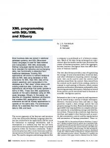
Sets, strings, and relations. The set of natural numbers is N = {0, 1, 2, . . . }. For m, n ∈ N, we denote the interval {k ∈ N | m ≤ k ≤ n} by [m, n]. The cardinality or size of a set A is denoted by #(A), and its powerset, i.e., the set of all its subsets, by 2A . The set of strings over A is denoted by A∗ . It consists of all sequences w = a1 · · · am with m ∈ N and ai ∈ A for every i ∈ [1, m]. The length m of w is denoted by |w|. The empty string (of length 0) is denoted by ε. The concatenation of two strings v and w is denoted by v · w or just vw. Moreover, w0 = ε and wn+1 = w · wn for n ∈ N. The composition of two binary relations R ⊆ A × B and S ⊆ B × C is R ◦ S = {(a, c) | ∃ b ∈ B : (a, b) ∈ R, (b, c) ∈ S}. The inverse of R is R−1 = {(b, a) | (a, S b) ∈ R}, and if A = B then the transitive-reflexive closure of R is R∗ = n∈N Rn where R0 = {(a, a) | a ∈ A} and Rn+1 = R ◦ Rn . The composition of two classes of binary relations R and S is R ◦ S = {R ◦ S | R ∈ R, S ∈ S}. Moreover, R1 = R and Rn+1 = R ◦ Rn for n ≥ 1. Trees and forests. An alphabet is a finite set of symbols. Let Σ be an alphabet, or an arbitrary set. Unranked trees and forests over Σ are recursively defined to be strings over the set Σ ∪ {(, )} consisting of the elements of Σ, the left parenthesis, and the right parenthesis, as follows. If σ ∈ Σ and t1 , . . . , tm are unranked trees, with m ∈ N, then their concatenation t1 · · · tm is a forest, and σ(t1 · · · tm ) is an unranked tree. For m = 0, t1 · · · tm is the empty forest ε. For readability we also write the tree σ(t1 · · · tm ) as σ(t1 , . . . , tm ), and even as σ when m = 0. Obviously, the concatenation of two forests is again a forest. It should also be noted that every nonempty forest can be written uniquely as σ(f1 )f2 where σ is in Σ and f1 and f2 are forests. The set of forests over Σ is denoted FΣ . For an arbitrary set A, disjoint with Σ, we denote by FΣ (A) the set all forests f over Σ ∪ A such that every node of f that is labelled by an element of A, is a leaf. As usual trees and forests are viewed as directed labelled graphs. Here we distinguish between two types of edges: “vertical” and “horizontal” ones. The root of the tree t = σ(t1 , . . . , tm ) is labelled by σ. It has vertical edges to the roots of subtrees t1 , . . . , tm , which are the children of the root of t and have child number 1 to m. The root of t is their parent. The roots of t1 , . . . , tm are siblings, also in the case of the forest t1 · · · tm . There is a horizontal edge from each sibling to the next, i.e., from the root of ti to the root of ti+1 for every i ∈ [1, m − 1]. Thus, the vertical edges represent the usual parent/child relationship, whereas the horizontal edges represent the linear order between children (and between the roots in a forest), see Fig. 1.3 For a tree t, its root 3 In

informal pictures the horizontal edges are usually omitted because they are implicit in

7

σ

τ

τ

a

b

b

a

σ

σ

a

b

a

τ

τ

b

b

a

σ

b

a

Figure 1: Picture of the forest σ(a, τ (b, a), b) τ (σ(a), b). Formal at the left, with dotted lines for the horizontal edges and solid lines for the vertical edges, and informal at the right. is denoted by roott , which is given child number 0 for technical convenience. Its set of nodes is denoted by N (t). For a forest f = t1 · · · tm , the set of nodes N (f ) is the disjoint union of the sets N (ti ), i ∈ [1, m]. For a node u of a tree t the subtree of t with root u is denoted t|u , and the i-th child of u is denoted ui (and similarly for a forest f instead of t). The nodes of a tree t correspond one-to-one to the positions of the elements of Σ in the string t, i.e., for every σ ∈ Σ, each occurrence of σ in t corresponds to a node of t with label σ. Since the positions of string t are naturally ordered from left to right, this induces an order on the nodes of t, which is called pre-order (or document order, when viewing t as an XML document). For example, the tree σ(τ (α, β), γ)) has five nodes which have the labels σ, τ , α, β, and γ in pre-order. A ranked alphabet (or set) Σ has an associated mapping rankΣ : Σ → N. The maximal rank of elements of Σ is denoted mxΣ . By Σ(m) we denote the elements of Σ with rank m. Ranked trees over Σ are recursively defined as above with the requirement that m = rankΣ (σ). The set of ranked trees over Σ is denoted TΣ . For an arbitrary set A, disjoint with Σ, we denote by TΣ (A) the set TΣ∪A where each element of A has rank 0. We will not consider ranked forests. Forests over an alphabet Σ can be encoded as binary trees, in the usual way: each node has a label in Σ, a “vertical” pointer to its first child, and a “horizontal” pointer to its next sibling; the pointer is nil if there is no such child or sibling. Such a binary tree can be modelled as a ranked tree over the ranked alphabet Σ ∪ {e} where every σ ∈ Σ has rank 2 and e is a symbol of rank 0 that represents the empty forest ε (or nil). Formally, the encoding of the empty forest equals enc(ε) = e, and recursively, the encoding enc(f ) of a forest f = σ(f1 )f2 equals σ(enc(f1 ), enc(f2 )). Obviously, enc is a bijection between forests over Σ and ranked trees over Σ ∪ {e}. The decoding which is its inverse will be denoted by dec. For an example of enc(f ) see Fig. 2 at the left. The disadvantage of this encoding is that the tree enc(f ) has more nodes than the forest f , viz. all nodes with label e. That is inconvenient when comparing the behaviour of tree-walking automata on f and enc(f ). Thus, we will also use an encoding that preserves the number of nodes (and thus cannot encode the empty forest). For this we use the ranked alphabet Σ′ consisting, for every the left-to-right orientation of the page. Similarly, the arrows of the vertical edges are omitted because of the top-down orientation of the page.

8

σ

σ 11

a

τ

e

τ

σ

b

e

e

a

b

a

e

e

e

e

b01

b

e

e

e

a01

τ 10

τ 11

σ 11

b00

a00

b00

a00

e

Figure 2: Encoding of the forest of Fig. 1 by enc (at the left) and by enc′ (at the right). σ ∈ Σ, of the symbols σ 11 of rank 2 (for a binary node without nil-pointers), σ 01 and σ 10 of rank 1 (for a binary node with vertical or horizontal nil-pointer, respectively), and σ 00 of rank 0 (for a binary node with two nil-pointers). The encoding enc′ (f ) of a nonempty forest f = σ(f1 )f2 equals σ 11 (enc′ (f1 ), enc′ (f2 )) or σ 01 (enc′ (f2 )) or σ 10 (enc′ (f1 )) or σ 00 , where the first (second) superscript of σ equals 0 if and only if f1 = e (f2 = e). Now, enc′ is a bijection between nonempty forests over Σ and ranked trees over Σ′ . The decoding which is its inverse will be denoted by dec′ . For an example of enc′ (f ) see Fig. 2 at the right. From the point of view of graphs, we assume that enc′ (f ) has the same nodes as f , i.e., N (enc′ (f )) = N (f ). The label of a node u of f is changed from σ to σ ij where i = 1 if and only if u has at least one child, and j = 1 if and only if u has a next sibling. If u has children, then its first child in enc′ (f ) is its first child in f , and its second child in enc′ (f ) is its next sibling (if it has one). If u has no children, then its only child in enc′ (f ) is its next sibling (if it has one). Although this encoding is intuitively clear, it is technically less attractive. We will use enc′ for the input forest of automata and transducers, and enc for the output forest of the transducers. We assume the reader to be familiar with the notion of a regular tree grammar. It is a context-free grammar G of which every rule is of the form X0 → σ(X1 · · · Xm ) where Xi is a nonterminal and σ is a terminal symbol of rank m. Thus, G generates a set L(G) of ranked trees, which is called a regular tree language. The class of regular tree languages will be denoted REGT. We define a regular forest grammar to be a context-free grammar G of which every rule is of the form X0 → σ(X1 )X2 or X → ε, where σ is from an unranked alphabet. It generates a set L(G) of (unranked) forests, which is called a regular forest language. Obviously, L is a regular forest language if and only if enc(L) is a regular tree language, and, as one can easily prove, if and only if enc′ (L) is a

9

regular tree language. The regular tree/forest grammar is a formal model of DTD (Document Type Definition) in XML.4 Monadic second-order logic (abbreviated as mso logic) is used to describe properties of forests and trees. It views each forest or tree as a logical structure that has the set of nodes as domain. As basic properties of a forest over alphabet Σ it uses the atomic formulas labσ (x), down(x, y), and next(x, y), meaning that node x has label σ ∈ Σ, that y is a child of x, and that y is the next sibling of x, respectively. Thus, down(x, y) and next(x, y) represent the vertical and horizontal edges of the graph representation of the forest. For a ranked tree over ranked alphabet Σ we could use the same atomic formulas, but it is customary to replace down(x, y) and next(x, y) by the atomic formulas downi (x, y), for every i ∈ [1, mxΣ ], meaning that y is the i-th child of x. Additionally, mso logic has the atomic formulas x = y and x ∈ X, where X is a set of nodes. The formulas are built with the usual connectives ¬, ∧, ∨, and →; both node variables x, y, . . . and node-set variables X, Y, . . . can be quantified with ∃ and ∀. For a forest (or ranked tree) f over Σ and a formula ϕ(x1 , . . . , xn ) with n free node variables x1 , . . . , xn , we write f |= ϕ(u1 , . . . , un ) to mean that ϕ holds in f for the nodes u1 , . . . , un of f (as values of the variables x1 , . . . , xn respectively). We will occasionally use the following formulas: root(x) and leaf(x) test whether node x is a root or a leaf, and first(x) and last(x) test whether x is a first or a last sibling. Also, childi (x) tests whether x is an i-th child, up(x, y) expresses that y is the parent of x, and stay(x, y) expresses that y equals x. Thus, we define stay(x, y) ≡ x = y and root(x) ≡ ¬ ∃z(down(z, x)), leaf(x) ≡ ¬ ∃z(down(x, z)), first(x) ≡ ¬ ∃z(next(z, x)), last(x) ≡ ¬ ∃z(next(x, z)), childi (x) ≡ ∃z(downi (z, x)), up(x, y) ≡ down(y, x). Patterns. Let Σ be a ranked alphabet and n ≥ 0. An n-ary pattern (or n-ary query) over Σ is a set T ⊆ {(t, u1 , . . . , un ) | t ∈ TΣ , u1 , . . . , un ∈ N (t)}. For n = 0 this is a tree language, for n = 1 it is a site (trees with a distinguished node), for n = 2 it is a trip [17] (or a binary tree-node relation [5]). We introduce a new ranked alphabet Σ×{0, 1}n, the rank of (σ, ℓ) equals that of σ in Σ. For a tree t over Σ and n nodes u1 , . . . , un we define mark(t, u1 , . . . , un ) to be the tree over Σ × {0, 1}n that is obtained by adding to the label of each node u in t a vector ℓ ∈ {0, 1}n such that the i-th component of ℓ equals 1 if and only if u = ui . The n-ary pattern T is regular if its marked representation is a regular tree language, i.e., mark(T ) ∈ REGT. An mso formula ϕ(x1 , . . . , xn ) over Σ, with n free node variables x1 , . . . , xn , defines the n-ary pattern T (ϕ) = {(t, u1 , . . . , un ) | t |= ϕ(u1 , . . . , un )}. Note that T (ϕ) also depends on the order x1 , . . . , xn of the free variables of ϕ. It easily follows from the result of Doner, Thatcher and Wright [10, 55] that a pattern is mso definable if and only if it is regular (see [5, Lemma 7]). We will also consider patterns on forests. For an unranked alphabet Σ, a (forest) pattern over Σ is a subset of {(f, u1 , . . . , un ) | f ∈ FΣ , u1 , . . . , un ∈ N (f )}. As for ranked trees, an mso formula ϕ(x1 , . . . , xn ) over Σ, defines the n-ary (forest) pattern {(f, u1 , . . . , un ) | f |= ϕ(u1 , . . . , un )}. 4 In

the litterature regular forest languages are usually defined in a different way, after which it is proved that L is a regular forest language if and only if enc(L) is a regular tree language, thus showing the equivalence with our definition, see, e.g., [46, Proposition 1].

10

3

Automata and Transducers

In this section we define tree-walking automata and transducers with pebbles, and discuss some of their properties. Automata. A tree-walking automaton with nested pebbles (pebble tree automaton for short, abbreviated pta) is a finite state device with one reading head that walks from node to node over its ranked input tree following the vertical edges in either direction. Additionally it has a supply of pebbles that can be used to mark the nodes of the tree. The automaton may drop a pebble on the node currently visited by the reading head, but it may only lift any pebble from the current node if that pebble was the last one dropped during the computation. Thus, the life times of the pebbles on the tree are nested. Here we consider two types of pebbles. First there are a finite number of “classical” pebbles, which we here call visible pebbles. Each of these has a distinct colour, and at most k visible pebbles (each with a different colour) can be present on the input tree during any computation, where k is fixed. Second there are invisible pebbles. Again, these pebbles have a finite number of colours (distinct from those of the visible pebbles), but for each colour there is an unlimited supply of pebbles that can be present on the input tree. Visible pebbles can be observed by the automaton at any moment when it visits the node where they were dropped. An invisible pebble can only be observed when it was the last pebble dropped on the tree during the computation. The possible actions of the automaton are determined by its state, the label of the current node, the child number of the node, and the set of observable pebbles on the current node, that is, visible pebbles and an invisible pebble when it was the last pebble dropped on the tree. Unlike the pta from [42], our automata do not branch (i.e., are not alternating). The pta is specified as a tuple A = (Σ, Q, Q0 , F, C, Cv , Ci , R, k), where Σ is a ranked alphabet of input symbols, Q is a finite set of states, Q0 ⊆ Q is the set of initial states, F ⊆ Q is the set of final states, Cv and Ci are the finite sets of visible and invisible colours, C = Cv ∪ Ci , Cv ∩ Ci = ∅, R is a finite set of rules, and k ∈ N. Each rule is of the form hq, σ, j, bi → hq ′ , αi such that q, q ′ ∈ Q, σ ∈ Σ, j ∈ [0, mxΣ ], b ⊆ C with #(b ∩ Cv ) ≤ k and #(b ∩ Ci ) ≤ 1, and α is one of the following instructions: stay, up downi dropc liftc

provided j 6= 0, with 1 ≤ i ≤ rankΣ (σ), with c ∈ C, and with c ∈ b,

where the first three are move instructions and the last two are pebble instructions. Note that, due to the nested life times of the pebbles, at most one pebble c in b can actually be lifted; however, the subscript c of liftc often increases the readability of a pta. A situation hu, πi of the pta A on ranked tree t over Σ is given by the position u of the head of A on t, and the stack π containing the positions and colours of the pebbles on the tree in the order in which they were dropped. Formally, u ∈ N (t) and π ∈ (N (t) × C)∗ . The last element of π represents the top of the stack. The set of all situations of A on t is denoted Sit(t), i.e., 11

Sit(t) = N (t) × (N (t) × C)∗ ; note that it only depends on C. A configuration hq, u, πi of A on t additionally contains the state q of A, q ∈ Q. It is final when q ∈ F . An initial configuration is of the form hq0 , roott , εi where q0 ∈ Q0 , roott is the root of t, and ε is the empty stack. The set of all configurations of A on t is denoted Con(t), i.e., Con(t) = Q × N (t) × (N (t) × C)∗ . We now define the computation steps of the pta A, which lead from one configuration to another. For a given input tree t they form a binary relation on Con(t). A rule hq, σ, j, bi → hq ′ , αi is relevant to every configuration hq, u, πi with state q and with a situation hu, πi that satisfies the tests σ, j, and b, i.e., σ and j are the label and child number of node u, and b is the set of colours of the observable pebbles dropped on the node u. More precisely, b consists of all c ∈ Cv such that (u, c) occurs in π, plus c ∈ Ci if (u, c) is the topmost (i.e., last) element of π. Application of the rule to such a configuration possibly leads to a new configuration hq ′ , u′ , π ′ i, in which case we write hq, u, πi ⇒t,A hq ′ , u′ , π ′ i. The new state is q ′ and the new situation hu′ , π ′ i is obtained from the situation hu, πi by the instruction α. For the move instructions α = stay, α = up, and α = downi the pebble stack does not change, i.e., π ′ = π, and the new node u′ equals u, is the parent of u, or is the i-th child of u, respectively. For the pebble instructions the node does not change, i.e., u′ = u. When α = dropc , A drops a pebble with colour c on the current node, thus the node-colour pair (u, c) is pushed onto the pebble stack π, i.e., π ′ = π(u, c), unless c is a visible colour and the stack already contains a pebble of that colour or already contains k visible pebbles, in which case the rule is not applicable.5 When α = liftc , A lifts a pebble with colour c from the current node, only allowed if the topmost element of the pebble stack is the pair (u, c), which is subsequently popped from the stack, i.e., π = π ′ (u, c); otherwise this rule is not applicable. We will also allow instructions like liftc ; up with the obvious meaning (first lift the pebble, then move up). In this way we have defined the binary relation ⇒t,A on Con(t), which represents the computation steps of M. We will say informally that a computation step of M halts successfully if it leads to a final configuration. The tree language L(A) accepted by pta A consists of all ranked trees t over Σ such that A has a successful computation on t that starts in an initial configuration. Formally, L(A) = {t ∈ TΣ | ∃ q0 ∈ Q0 , q∞ ∈ F, hu, πi ∈ Sit(t) : hq0 , roott , εi ⇒∗t,A hq∞ , u, πi}. Note that pebbles may remain in the final configuration and that the head need not return to the root. Two pta’s A and B are equivalent if L(A) = L(B). By vk i-pta we denote a pta with last component k, i.e., that uses at most k visible pebbles in its computations, and an unbounded number of invisible pebbles, and by Vk I-PTA we denote the class of tree languages accepted by vk i-pta’s. For k = 0, automata that only use invisible pebbles, we also use the notation i-pta, and for automata that only use k visible pebbles we use vk -pta. Moreover, ta is used for tree-walking automata without pebbles, i.e., v0 -pta. The lower case d or d is added when we only consider deterministic automata, which have a unique initial state, no final state in the left-hand side of a rule, and no two rules with the same left-hand side. Thus we have vk i-dpta, Vk I-dPTA, and variants.

5 To be precise, the rule is not applicable if c ∈ C , π = (u , c ) · · · (u , c ), and there v n n 1 1 exists i ∈ [1, n] such that c = ci , or #({i ∈ [1, n] | ci ∈ Cv }) = k.

12

Properties of automata. It is natural, and sometimes useful, to extend the vk i-pta with the facility to test whether its pebble stack is nonempty, and if so, to test the colour of the topmost pebble. Thus, we define a pta with stack tests in the same way as an ordinary pta except that its rules are of the form hq, σ, j, b, γi → hq ′ , αi with γ ∈ C ∪{ε}. Such a rule is relevant to a configuration hq, u, πi if, in addition, the pebble stack π is empty if γ = ε, and the topmost pebble of π has colour γ if γ ∈ C.6 All other definitions are the same. Note that, obviously, we may require for the above rule that γ = c if α = liftc , which ensures that relevant rules with a lift-instruction are always applicable.7 It is not difficult to see that these new tests do not extend the expressive power of the pta. Informally we will say that the vk i-pta can perform stack tests. Lemma 1 Let k ≥ 0. For every vk i-pta with stack tests A an equivalent (ordinary) vk i-pta A′ can be constructed in polynomial time. The construction preserves determinism and the absence of invisible pebbles.8 Proof. Let A = (Σ, Q, Q0 , F, C, Cv , Ci , R, k). The new automaton A′ stepwise simulates A and, additionally, stores in its finite state whether or not the pebble stack is nonempty, and if so, what is the colour in C of the topmost pebble. Thus, Q′ = Q×(C ∪{ε}), Q′0 = Q0 ×{ε}, and F ′ = F ×(C ∪{ε}). Moreover, the colour sets of A′ are Cv′ = Cv × (C ∪ {ε}) and Ci′ = Ci × (C ∪ {ε}). In fact, if the pebble stack of A is π = (u1 , c1 )(u2 , c2 ) · · · (un , cn ), with (un , cn ) being the topmost pebble, then the stack of A′ is π ′ = (u1 , (c1 , ε))(u2 , (c2 , c1 )) · · · (un , (cn , cn−1 )), where ε is viewed as a bottom symbol. Thus, the new colour of a pebble contains its old colour together with the old colour of the previously dropped pebble (or ε if there is none). This allows A′ to update its additional finite state component when A lifts a pebble. More precisely, when A is in configuration hq, u, πi, the automaton A′ is in configuration h(q, γ), u, π ′ i, where γ = cn if n ≥ 1 and γ = ε otherwise. The rules of A′ are defined as follows. Let hq, σ, j, b, γi → hq ′ , αi be a rule of A, and let b′ be (the graph of) a mapping from b to C ∪ {ε}. If α is a move instruction, then A′ has the rule h(q, γ), σ, j, b′ i → h(q ′ , γ), αi. If α = dropc , then A′ has the rule h(q, γ), σ, j, b′ i → h(q ′ , c), drop(c,γ) i. If α = liftc , γ = c, and (c, γ ′ ) ∈ b′ , then A′ has the rule h(q, γ), σ, j, b′ i → h(q ′ , γ ′ ), lift(c,γ ′ ) i. It should be clear that the construction of A′ takes polynomial time. Note that k is fixed and #(b) ≤ k + 1 in the left-hand side of the rule hq, σ, j, b, γi → hq ′ , αi of A. ✷ pta’s with stack tests will only be used in Sections 8 and 15. The next two properties of pta’s will not be used in later sections, but are meant to clarify some of the details in the semantics of the pta. A rule of a vk i-pta A is progressive if it is applicable to every reachable configuration9 to which it is relevant. The vk i-pta A is progressive if all its 6 To be precise, for π = (u , c ) · · · (u , c ) the requirements are the following: If γ = ε n n 1 1 then n = 0, i.e., π = ε. If γ ∈ C then n ≥ 1 and cn = γ. 7 Additionally, we can require the following: If γ = ε then b = ∅. If b ∩ C = {c} then i γ = c. 8 In other words, the statement of the lemma also holds for v i-dpta, v -pta and v -dpta. k k k 9 The configuration hq, u, πi on the tree t is reachable if hq , root , εi ⇒∗ t 0 t,A hq, u, πi for some q0 ∈ Q0 .

13

rules are progressive. Intuitively this means that A knows that its instructions can always be executed. Clearly, according to the syntax of a pta, every rule with a move instruction is progressive. The same is true for rules with a pebble instruction dropc or liftc with c ∈ Ci : an invisible pebble can always be dropped and an observable invisible pebble can always be lifted. Thus, only the dropping and lifting of visible pebbles is problematic. It is easy to see that, for the vk i-pta A′ constructed in the proof of Lemma 1, every rule with a lift-instruction is progressive. A vk i-pta A is counting if Cv = [1, k] and, in each reachable configuration, the colours of the visible pebbles on the tree are 1, . . . , ℓ for some ℓ ∈ [0, k], in the order in which they were dropped.10 Note that in the litterature vk -pta’s are usually counting. We have chosen to allow arbitrarily many visible colours in a vk i-pta because we want to be able to store information in the pebbles, as in the proof of Lemma 1. It is straightforward to construct an equivalent counting vk i-pta A′ for a given vk i-pta A (preserving determinism and the absence of invisible pebbles). The automaton A′ stepwise simulates A and, additionally, stores in its finite state the colours of the visible pebbles that are dropped on the tree, in the order in which they were dropped. Thus, the states of A′ are of the form (q, ϕ) where q is a state of A and ϕ is a string over Cv without repetitions, of length at most k. The state (q, ϕ) is final if q is final. The initial states are (q, ε) where q is an initial state of A. The rules of A′ are defined as follows. Let hq, σ, j, bi → hq ′ , αi be a rule of A and let (q, ϕ) be a state of A′ such that every c ∈ b ∩ Cv occurs in ϕ. Moreover, let b′ ⊆ [1, k] ∪ Ci be obtained from b by changing every c ∈ Cv into i, if c is the i-th element of ϕ. If α is a move instruction, or a pebble instruction dropc or liftc with c ∈ Ci then A′ has the rule h(q, ϕ), σ, j, b′ i → h(q ′ , ϕ), αi. If α = dropc with c ∈ Cv , c does not occur in ϕ, and |ϕ| < k, then A′ has the rule h(q, ϕ), σ, j, b′ i → h(q ′ , ϕc), drop|ϕ|+1 i. Finally, if α = liftc with c ∈ Cv , and ϕ = ϕ′ c for some ϕ′ ∈ Cv∗ , then A′ has the rule h(q, ϕ), σ, j, b′ i → h(q ′ , ϕ′ ), lift|ϕ| i. It should be clear that A′ is counting. Note also that all rules of A′ with a drop-instruction are progressive. Thus, if we first apply the construction in the proof of Lemma 1 and then the one above, we obtain an equivalent progressive vk i-pta. Obviously, every progressive vk i-pta can be turned into an equivalent vk+1 i-pta by simply changing its last component k into k + 1, and hence Vk I-PTA ⊆ Vk+1 I-PTA and Vk I-dPTA ⊆ Vk+1 I-dPTA.11 Transducers. A tree-walking tree transducer with nested pebbles (abbreviated ptt) is a pta without final states that additionally produces an output tree over a ranked alphabet ∆. Thus, omitting F , it is specified as a tuple M = (Σ, ∆, Q, Q0 , C, Cv , Ci , R, k), where Σ, Q, Q0 , C, Cv , Ci , and k are as for the pta. The rules of M in the finite set R are of the same form as for the pta, except that M additionally has output rules of the form hq, σ, j, bi → δ( hq1 , stayi, . . . , hqm , stayi ) with δ ∈ ∆, and q1 , . . . , qm ∈ Q, where m is the rank of δ. Intuitively, the output tree is produced recursively. In other words, in a configuration to which the above output rule is relevant (defined as for the pta) the ptt M outputs δ, and for each child hqi , stayi branches into a new process, a copy of itself started in state qi at the current 10 To be precise, for π = (u , c ) · · · (u , c ) we require that there exists ℓ ∈ [0, k] such that n n 1 1 (ci1 , . . . , cim ) = (1, . . . , ℓ) where {i1 , . . . , im } = {i ∈ [1, n] | ci ∈ Cv } and i1 < · · · < im . 11 In fact, these four classes are equal, as will be shown in Theorem 11.

14

node, retaining the same stack of pebbles; thus, the stack is copied m times. Note that a relevant output rule is always applicable. As a shortcut we may replace the stay-instruction in any hqi , stayi by another move instruction or a pebble instruction, with obvious semantics. An output form of the ptt M on ranked tree t over Σ is a tree in T∆ (Con(t)), where Con(t) is defined as for the pta. Intuitively, such an output form consists on the one hand of ∆-labeled nodes that were produced by M previously in the computation, using output rules, and on the other hand of leaves that represent the independent copies of M into which the computation has branched previously, due to those output rules, where each leaf is labeled by the current configuration of that copy. Note that Con(t) ⊆ T∆ (Con(t)), i.e., every configuration of M is an output form. The computation steps of the ptt M lead from one output form to another. Let s be an output form and let v be a leaf of s with label hq, u, πi ∈ Con(t). If hq, u, πi ⇒t,M hq ′ , u′ , π ′ i, where the binary relation ⇒t,M on Con(t) is defined as for the pta (disregarding the output rules of M), then we write s ⇒t,M s′ where s′ is obtained from s by changing the label of v into hq ′ , u′ , π ′ i. Moreover, for every output rule hq, σ, j, bi → δ( hq1 , stayi, . . . , hqm , stayi ) that is relevant to configuration hq, u, πi, we write s ⇒t,M s′ where s′ is obtained from s by replacing the node v by the subtree δ(hq1 , u, πi, . . . , hqm , u, πi). In the particular case that m = 0, s′ is obtained from s by changing the label of v into δ. In that case we will say informally that M halts successfully, meaning that the copy of M corresponding to the node u of s disappears. In this way we have extended ⇒t,M to a binary relation on T∆ (Con(t)). The transduction τM realized by M consists of all pairs of trees t over Σ and s over ∆ such that M has a (successful) computation on t that starts in an initial configuration and ends with s. Formally, we define τM = {(t, s) ∈ TΣ × T∆ | ∃ q0 ∈ Q0 : hq0 , roott , εi ⇒∗t,M s}. Two ptt’s M and N are equivalent if τM = τN . The domain of M is defined to be the domain of τM , i.e., the tree language L(M) = {t ∈ TΣ | ∃ s ∈ T∆ : (t, s) ∈ τM }. When M is viewed as a recognizer of its domain, it is actually the same as an alternating pta. Existential states in the alternation correspond to the nondeterminism of the ptt, universal states correspond to the recursive way in which output trees are generated. More precisely, an output rule hq, σ, j, bi → δ( hq1 , stayi, . . . , hqm , stayi ) corresponds to a universal state q that requires every state qi to have a successful computation (and the output symbol δ is irrelevant). An ordinary (non-alternating) pta then corresponds to a ptt for which every output symbol has rank 0; for m = 0 the above output rule means that the pta halts in a final state. We say that the ptt M is total if L(M) = TΣ , i.e., τM (t) 6= ∅ for every input tree t. Similar to the notation Vk I-PTA for tree languages, we use the notation Vk I-PTT for the class of transductions defined by tree-walking tree transducers with k visible nested pebbles and an unbounded number of invisible pebbles, as well as the obvious variants Vk -PTT, and I-PTT. Additionally TT denotes the class of transductions realized by tree-walking tree transducers without pebbles, i.e., V0 -PTT. Such a transducer is specified as a tuple M = (Σ, ∆, Q, Q0 , R), and the left-hand sides of its rules are written hq, σ, ji, omitting b = ∅. As for pta’s, lower case d is added for deterministic transducers, which have a unique initial state and no two rules with the same left-hand side. Moreover, lower case td is used for total deterministic transducers, i.e., transducers that are both total 15

and deterministic. Note that a deterministic ptt realizes a function, and a total deterministic ptt a total function from TΣ to T∆ . Properties of transducers. Stack tests are defined for the ptt as for the pta, and Lemma 1 and its proof carry over to ptt’s. If a given ptt M has the output rule hq, σ, j, b, γi → δ(hq1 , stayi, . . . , hqm , stayi), and b′ is (the graph of) a mapping from b to C ∪ {ε} as in the proof for pta’s, then the constructed ptt M′ has the rule h(q, γ), σ, j, b′ i → δ(h(q1 , γ), stayi, . . . , h(qm , γ), stayi). Progressive ptt’s can be defined as for pta’s, based on the notion of a reachable configuration, cf. footnote 9. An output form s of the ptt M on the input tree t is reachable if hq0 , roott , εi ⇒∗t,M s for some q0 ∈ Q0 . A configuration of M on t is reachable if it occurs in some reachable output form of M on t. Note that every i-ptt is progressive. Also, counting ptt’s can be defined as for pta’s. For every vk i-ptt M an equivalent counting vk i-ptt M′ can be constructed, just as for pta’s. If hq, σ, j, b, γi → δ(hq1 , stayi, . . . , hqm , stayi) is an output rule of M, and ϕ and b′ are as in the proof for pta’s, then M′ has the rule h(q, ϕ), σ, j, b′ i → δ(h(q1 , ϕ), stayi, . . . , h(qm , ϕ), stayi). Thus, as for pta’s, every vk i-ptt can be turned into an equivalent progressive vk i-ptt, with determinism and the absence of invisible pebbles preserved. That implies that Vk I-PTT ⊆ Vk+1 I-PTT and Vk I-dPTT ⊆ Vk+1 I-dPTT. We end this section with an example of an i-ptt. Example 2 We want to generate itineraries for a trip along the Trans-Siberian Railway, starting in Moscow and ending in Vladivostok, and optionally visiting some cities along the way. An XML document lists all the stops: ... ... ... ...

The initial and final stops are marked, and for every stop the large attribute indicates whether or not the stop is in a large city. We want to generate a list it-1 it-2 ... it-n ...

where it-1,it-2,...,it-n are all itineraries (i.e., lists of stops) that satisfy the constraint that one does not visit a small city twice in a row. An example input XML document, with the corresponding output XML document is given in Tables 1 and 2 (where, e.g., ^3 abbreviates ). 16

A deterministic i-ptt Msib is able to perform this XML transformation by systematically enumerating all possible lists of stops, marking each stop in the list (except the initial and final stop) by a pebble. Since the pebbles are invisible, Msib constructs a possible list of stops on the pebble stack in reverse, so that the stops will appear in the output tree in the correct order. ^5

Table 1: Input Since in this example the XML tags are ranked, there is no need for a binary encoding of the XML documents. The input alphabet Σ of Msib consists of all where at is a possible value of the attributes. The rank of is 0 if final="1" and 1 otherwise. The output alphabet ∆ consists of Σ, the tag r = of rank 2, and the tag e = of rank 0. The set of pebble colours is C = Ci = {0, 1}, with Cv = ∅. The transducer Msib will not use the attribute initial, as it can recognize the root by its child number 0. Also, it will disregard the attribute large of the initial and the final stop, and always consider them as large cities. The set of states of Msib is Q = {qstart , q1 , q0 , qout , qnext } with Q0 = {qstart }. In the rules below the variables range over the following values: σ0 ∈ Σ(0) , σ1 ∈ Σ(1) , j, c ∈ {0, 1}, and, for i ∈ {0, 1}, λi ∈ { ∈ Σ | large="i"}. The i-ptt Msib first walks from Moscow to Vladivostok in state qstart : hqstart , σ1 , j, ∅i → hqstart , down1 i hqstart , σ0 , 1, ∅i → hq1 , upi State qc remembers whether the most recently marked city is small or large; when a new city is marked with a pebble, it gets the colour c. In states q0 and q1 as many cities are marked as possible (in the second rule, c = 1 or i = 1): hq0 , λ0 , 1, ∅i → hq0 , upi hqc , λi , 1, ∅i → hqi , dropc ; upi hqc , σ1 , 0, ∅i → r(hqout , stayi, hqnext , down1 i) In state qout an itinerary is generated as output, while state qnext continues the search for itineraries by unmarking the most recently marked city: hqout , σ1 , 0, ∅i → σ1 (hqout , down1 i) hqout , σ1 , 1, ∅i → hqout , down1 i hqout , σ1 , 1, {c}i → σ1 (hqout , liftc ; down1 i) hqout , σ0 , 1, ∅i → σ0 hqnext , σ1 , 1, ∅i → hqnext , down1 i hqnext , σ1 , 1, {c}i → hqc , liftc ; upi hqnext , σ0 , 1, ∅i → e

17

^4 ^4 ^3 ^2 ^3 ^3 ^2 ^2 ^2 ^8

Table 2: Output

18

Note that this XML transformation cannot be realized by a v-ptt, because the height of the output tree is, in general, exponential in the size of the input tree, whereas it is polynomial for v-ptt’s (cf. [20, Lemma 7]). ✷

4

Decomposition

In this section we decompose every ptt into a sequence of tt’s, i.e., transducers without pebbles. This is useful as it will give us information on the domain of a ptt, see Theorem 11, and on the complexity of typechecking the ptt, see Theorem 8. It is possible to reduce the number of visible pebbles used, by preprocessing the input tree with a total deterministic tt. This was shown in [20, Lemma 9] for transducers with only visible pebbles. The basic idea of that proof can be extended to include invisible pebbles. Lemma 3 Let k ≥ 1. For every vk i-ptt M a total deterministic tt N and a vk−1 i-ptt M′ can be constructed in polynomial time such that τN ◦ τM′ = τM . If M is deterministic, then so is M′ . Hence, for every k ≥ 1, Vk I-PTT ⊆ tdTT ◦ Vk−1 I-PTT and Vk I-dPTT ⊆ tdTT ◦ Vk−1 I-dPTT. Proof. Let M = (Σ, ∆, Q, Q0 , C, Cv , Ci , R, k) be a ptt with k visible pebbles. The construction of the tt N and the ptt M′ with k − 1 visible pebbles is a straightforward extension of the one in [13, Theorem 5], which slightly differs from the one in the proof of [20, Lemma 9], but uses the same basic idea. For completeness sake we repeat a large part of the proof of [13, Theorem 5], adapted to the current formalism. The simple idea of the proof is to preprocess the input tree t ∈ TΣ in such a way that the dropping and lifting of the first visible pebble can be simulated by walking into and out of specific areas of the preprocessed input tree pp(t). This preprocessing is independent of the given pebble tree transducer M. More precisely, pp(t) is obtained from t by attaching to each node u of t, as an additional (last) subtree, a fresh copy of t in which (the copy of) node u is marked; let us denote this subtree by tu . Thus, if t has n nodes, then pp(t) has n + n2 nodes. The subtrees tu of pp(t) are the “specific areas” mentioned above. As long as there are no visible pebbles on t, M′ stepwise simulates M on the original nodes of t, which form the “top level” of pp(t). When M drops the first visible pebble c on node u, M′ enters tu and walks to the marked node, storing c in its finite state. As long as M keeps pebble c on the tree, M′ stays in tu , stepwise simulating M on tu rather than t. Since u is marked in tu , M’s pebble c at u is visible to the transducer M′ , not as a pebble but as a marked node. Thus, during this time, M′ only uses k − 1 visible pebbles. When M lifts pebble c from u (and hence all visible pebbles are lifted), M′ walks from the copy of u out of tu , back to the original node u, and continues simulating M on the top level of pp(t) until M again drops a visible pebble. There is one problem: how does M′ know whether or not pebble c is on top of the stack when M tries to lift it? To solve this problem, M′ uses an additional special invisible pebble ⊙. It drops pebble ⊙ at the copy of u and thus knows that pebble c is at the top of the stack (for M) when it observes pebble ⊙. Thus, at any moment of time, M′ has the same pebble stack as M,

19

except that c is replaced by ⊙ and, moreover, the (invisible) pebbles below ⊙ are on the top level of pp(t), whereas ⊙ and the pebbles above it are on tu . Unfortunately, this preprocessing cannot be realized by a tt (though it can easily be realized by a v1 -ptt). For this reason we “fold” tu at the node u, such that (the marked copy of) u becomes its root; let us denote the resulting tree by tˆu . Roughly, tˆu is obtained from tu by inverting the parent-child relationship between the ancestors of u (including u), similarly as in the tree traversal algorithm sometimes known as “link inversion” [35, p.562]. Appropriate information is added to the node labels of those ancestors to reflect this inversion. As these changes are local (i.e., each node keeps the same neighbours) and clearly marked in the tree, M′ can easily reconstruct the unfolded tu , and simulate M as before. Note also that, with this change of pp(t), dropping or lifting of the first visible pebble can be simulated by M′ in one computation step, because the marked copy of u is the last child of the original u. Now a tt N can compute pp(t), as follows12 . It copies t to the output (adding primes to its labels), but when it arrives at node u it additionally outputs the copy tˆu of t in a side branch of the computation. Copying the descendants of u “down stream” is an easy recursive task. To invert the parentchild relationship between the nodes on the path from u to roott , N uses a single process that walks along the nodes of that path “up stream” to the root, inverting the relationships in the copy. Copies of other siblings of children on the path are connected as in t, and their descendants are copied “down stream”. More precisely, if in t the i-th child v of parent w is on the path, then, in the output tˆu , v has an additional (last) child that corresponds to w, and w has the same children (with their descendants) as in t, except that its i-th child is a node that is labeled by the bottom symbol ⊥ of rank 0. For the sake of uniformity, roott is also given an additional (last) child, with label ⊥. Note that the nodes of t correspond one-to-one to the non-bottom nodes of tˆu ; in particular, the path in t from u to roott corresponds to the path in tˆu from its root to the parent of its rightmost leaf. The bottom nodes of tˆu will not be visited by M′ . A picture of pp(t) is given in Fig. 3, where tˆu is drawn for two nodes only. Note that in this picture the root of the copy of t (which is also the root of pp(t)) is the top of the triangle, but the root of tˆu is u (and, of course, similarly for v). As a concrete example, consider t = σ(δ(a, b), c) where σ, δ have rank 2 and a, b, c rank 0. We will name the nodes of t by their labels. Then pp(t) = σ ′ (δ ′ (a′ (tˆa ), b′ (tˆb ), tˆδ ), c′ (tˆc ), tˆσ ) where

tˆa tˆb tˆδ tˆc tˆσ

= = = = =

a0,1 (δ1,1 (⊥, b, σ1,0 (⊥, c, ⊥))), b0,2 (δ2,1 (a, ⊥, σ1,0 (⊥, c, ⊥))), δ0,1 (a, b, σ1,0 (⊥, c, ⊥)), c0,2 (σ2,0 (δ(a, b), ⊥, ⊥)), and σ0,0 (δ(a, b), c, ⊥).

The subscripted node labels are on the rightmost paths of the tˆu ’s; the subscripts contain “reconstruction” information, to be explained below. As another example, if t is the monadic tree a(bm (c(dn (e)))) of height m + n + 3, and u is the 12 See also [42, Example 3.7] where tˆ occurs as “a complex rotation of the input tree” t, u albeit for leaves u only.

20

t

v tˆu

tˆv

u v

u Figure 3: Output tree pp(t) of the tt N of Lemma 3 for input tree t. c-labelled node, then tˆu = c0,1 (s1 , s2 ) with s1 = dn (e) and s2 is the binary tree b1,1 (⊥, b1,1 (⊥, . . . b1,1 (⊥, a1,0 (⊥, ⊥)) · · · )) of height m + 2. This shows more clearly that tˆu is obtained by “folding”. We now formally define the deterministic tt N that, for given ranked alphabet Σ, realizes the preprocessing pp (called EncPeb in [20]). The definition is identical to the one in [13, Section 6]. Since N has no pebbles, we abbreviate the left-hand side hq, σ, j, ∅i of a rule by hq, σ, ji. To simplify the definition of N we additionally allow output rules of the form hq, σ, ji → δ(s1 , . . . , sm ) where δ is an output symbol of rank m and every si is either the output symbol ⊥ or it is of the form hq ′ , ϕi where ϕ is stay, up, or downi with i ∈ [1, m]. Such a rule should be replaced by the rules hq, σ, ji → δ(hp1 , stayi, . . . , hpm , stayi) and hpj , σ, ji → sj for all j ∈ [1, m], where p1 , . . . , pm are new states. Obviously this replacement can be done in quadratic time. We introduce the states and rules of N one by one; in what follows σ ranges over Σ, with m = rankΣ (σ), j ranges over [0, mxΣ ], and i over [1, m]. First, N has an “identity” state d that just recursively copies the subtree of the current node to the output, using the rules hd, σ, ji → σ(hd, down1 i, . . . , hd, downm i). Then, N has initial state g that copies the input tree t to the output (with primed labels) and at each node u of t “generates” a new copy tˆu of the input tree by calling the state f that computes tˆu by “folding” tu . The rules for g are hg, σ, ji → σ ′ (hg, down1 i, . . . , hg, downm i, hf, stayi). Note that σ ′ has rank m + 1: the root of tˆu is attached to u as its last child. The rules for f are hf, σ, ji → σ0,j (hd, down1 i, . . . , hd, downm i, ξj ) where ξj = hfj , upi for j 6= 0, and ξ0 = ⊥. The “reconstruction” subscripts of σ0,j mean the following: subscript 0 indicates that this node is the root of some tˆu , and subscript j is the child number of u in t. Note that σ0,j has rank m + 1: its last child corresponds to the parent of u in t (viewing ⊥ as the “parent” of roott in t). The tt N walks up along the path from u to the root of t using “folding” states fi , where the i indicates that in the previous step N was at the

21

i-th child of the current node. The rules for fi are hfi , σ, ji

→ σi,j ( hd, down1 i, . . . , hd, downi−1 i, ⊥, hd, downi+1 i, . . . , hd, downm i, ξj )

where ξj is as above. If a node (in tˆu ) with label σi,j corresponds to the node v in t, then the “reconstruction” subscript i means that its parent corresponds to the i-th child of v in t (and its own i-th child is ⊥), and, as above, “reconstruction” subscript j is the child number of v. Just as σ0,j , also σi,j has rank m + 1: its last child corresponds to the parent of v in t. Note that the copy tˆu of the input tree is computed by the states f , fi (for every i) and d, such that f copies node u to the output and the other states walk from u to every other node v of t and copy v to the output. To be precise, N walks from u to v along the shortest (undirected) path from u to v, from u up to the least common ancestor of u and v (in the states fi ), and then down to v (in the state d). Arriving in a node v from a neighbour of v, the transducer N branches into a new process for every other neighbour of v. This ends the description of the tt N . The output alphabet Γ of N (which will also be the input alphabet of M′ ) is the union of Σ, {⊥}, {σ ′ | σ ∈ Σ}, and {σi,j | σ ∈ Σ, i ∈ [0, rankΣ (σ)], j ∈ [0, mxΣ ]}. Thus, N has O(n2 ) output symbols, where n is the size of Σ.13 So, since mxΓ = mxΣ + 1, the size of Γ is polynomial in n. The set of states of N is {d, g, f } ∪ {fi | i ∈ [1, mxΣ ]}, with initial state g. Thus, it has O(n) states and O(n3 ) rules; moreover, each of these rules is of size O(n log n). Hence, the size of N is polynomial in the size of Σ, and it can be constructed in polynomial time. We now turn to the description of the vk−1 i-ptt M′ . It has input alphabet Γ, output alphabet ∆, set of states Q ∪ (Q × Cv ), and the same initial states and visible colours as M. Its invisible colour set is Ci′ = Ci ∪ {⊙}. It remains to discuss the set R′ of rules of M′ . Let hq, σ, j, bi → ζ be a rule of M with rankΣ (σ) = m. We consider four cases, depending on the variant σ ′ , σ0,j , σi,j with i 6= 0, or σ in Γ of the input symbol σ ∈ Σ. In the first case, we consider the behaviour of M′ in state q on σ ′ , and we assume that b ∩ Cv = ∅. If ζ = hq ′ , dropc i with c ∈ Cv , then R′ contains the rule hq, σ ′ , j, bi → h(q ′ , c), downm+1 ; drop⊙ i,14 and otherwise R′ contains the rule hq, σ ′ , j, bi → ζ. Thus, M′ simulates M on the original (now primed) part of the input tree t in pp(t), until M drops a visible pebble c on node u. Then M′ steps to the root of tˆu where it drops the invisible pebble ⊙, and stores c in its finite state. Next, we let c ∈ Cv and we consider the behaviour of M′ in state (q, c) on the remaining variants of σ. Let ζc be the result of changing in ζ every occurrence of a state q ′ into (q ′ , c). In the second case we assume that c ∈ b (corresponding to the fact that σ0,j labels the marked node of some tˆu ). If b = {c} and ζ = hq ′ , liftc i, then 13 We assume here that the rank of each symbol of the ranked alphabet Σ is specified in unary rather than decimal notation, and thus mxΣ ≤ n; cf. the last paragraph of [13, Section 2]. 14 To be completely formal, this rule should be replaced by the two rules hq, σ ′ , j, bi → hp, downm+1 i and hp, σ0,j , m + 1, ∅i → h(q ′ , c), drop⊙ i, where p is a new state.

22

R′ contains the rule h(q, c), σ0,j , m + 1, {⊙}i → hq ′ , lift⊙ ; upi.15 Thus, when M lifts visible pebble c from node u, M′ lifts invisible pebble ⊙ and steps from the root of tˆu back to node u. Otherwise, R′ contains the rules h(q, c), σ0,j , m + 1, b \ {c} ∪ {⊙}i → ζc′ (provided b ∩ Ci = ∅) and h(q, c), σ0,j , m + 1, b \ {c}i → ζc′ , where ζc′ is obtained from ζc by changing up into downm+1 . These two rules correspond to whether or not the invisible pebble ⊙ is observable. Note that the child number in pp(t) of a node with label σ0,j is always m + 1 (and the label of its parent is σ ′ ). In the remaining two cases we assume that c ∈ / b in the above rule of M. In the third case, we consider σi,j with i 6= 0. Then R′ contains the rules h(q, c), σi,j , j ′ , bi → ζc′ for every j ′ ∈ [1, mxΓ ], where ζc′ is now obtained from ζc by changing up into downm+1 , and downi into up. In the fourth and final case, we consider σ itself (in Γ). Then R′ contains the rule h(q, c), σ, j, bi → ζc . Thus, M′ stepwise simulates M on every tˆu . This ends the description of the vk−1 i-ptt M′ . It should now be clear that τM′ (pp(t)) = τM (t) for every t ∈ TΣ , and hence τN ◦ τM′ = τM . Each rule of M is turned into at most 1 + #(Cv ) · (2 + mxΣ (mxΣ + 1)) rules of M′ , of the same size as that rule (disregarding the space taken by the occurrences of c and m + 1). Thus, M′ can be computed from M in polynomial time. ✷ The tree pp(t) that is used in the previous proof consists of two levels of copies of the original input tree t; on the first level a straightforward copy of t (used until the first visible pebble is dropped) and a second level of copies tˆu (used to “store” the first visible pebble dropped). It is tempting to add another level, meant as a way to store the next visible pebble dropped. The problem with this is that it would make the first visible pebble effectively unobservable when the next one is dropped. The idea can be used for invisible pebbles, for arbitrarily many levels. Lemma 4 For every i-ptt M a tt N and a tt M′ can be constructed in polynomial time such that τN ◦ τM′ = τM . If M is deterministic, then so is M′ . Hence, I-PTT ⊆ TT ◦ TT and I-dPTT ⊆ TT ◦ dTT. Proof. The computation of a ptt M with invisible pebbles on tree t is simulated by a tt M′ (without pebbles) on tree t′ . The input tree t is preprocessed in a nondeterministic way by a tt N to obtain t′ . The top level of t′ is a copy of t, as before. On the next level, since the simulating transducer M′ cannot store the colours of all the pebbles in its finite state (as we did for one colour in the proof of Lemma 3), N does not attach one copy tˆu of t to each node u of t but #(Ci ) such copies, one for each pebble colour. In this way, the child number in t′ of the root of tˆu represents the pebble colour. In fact, in each node u of t the transducer N nondeterministically decides for each pebble colour c whether 15 Again, to be completely formal, this rule should be replaced by the two rules h(q, c), σ0,j , m + 1, {⊙}i → hp, lift⊙ i and hp, σ0,j , m + 1, ∅i → hq ′ , upi, where p is a new state.

23

t

Figure 4: An output tree t′ of the tt N of Lemma 4 for input tree t. or not to spawn a process that copies t into tˆu , and this is a recursive process: in each node in each copy of t it can be decided to spawn such processes that generate new copies. In this way a “tree of trees” is constructed. For an “artist impression” of such an output tree t′ , see Fig. 4. The child number in t′ of the root of each copy tˆu indicates an invisible pebble of colour c placed at node u in the original tree t. In each copy only one pebble is observable, the one represented by the child number of its root, exactly as the last pebble dropped in the original computation. In the simulation, moving down or up along the tree of trees corresponds to dropping and lifting invisible pebbles. In general there is no bound on the depth of the stack of pebbles during a computation of M. The preprocessor N nondeterministically constructs t′ . If t′ is not sufficiently deep, the simulating transducer M′ aborts the computation. Conversely, for every computation of M a tree t′ of sufficient depth can be constructed nonderministically from t. We now turn to the formal definitions. Let M = (Σ, ∆, Q, Q0 , C, Cv , Ci , R, 0) be an i-ptt. Without loss of generality we assume that C = Ci and that C = [1, γ] for some γ ∈ N. This choice of C simplifies the representation of colours by child numbers. First, we define the nondeterministic tt N that preprocesses the trees over Σ. It is a straightforward variant of the one in the proof of Lemma 3. The output alphabet Γ of N is now the union of {⊥}, {σ ′ | σ ∈ Σ}, and ′ {σi,j | σ ∈ Σ, i ∈ [0, rankΣ (σ)], j ∈ [0, mxΣ ]} where, for every σ ∈ Σ of rank m, ′ ′ has rank m + γ + 1, because γ processes are spawned σ has rank m + γ and σi,j at each node, and each of these processes generates, nondeterministically, either a copy tˆu of t or the bottom symbol ⊥. The set of states of N is as before, except that the state d is removed (with its rules). In the rules of N we will use hf, stayiγ as an abbreviation of the sequence hf, stayi, . . . , hf, stayi of length γ. The rules for the initial state g are hg, σ, ji → σ ′ (hg, down1 i, . . . , hg, downm i, hf, stayiγ ).

24

The rules for f are hf, σ, ji hf, σ, ji

→ ⊥ ′ → σ0,j (hg, down1 i, . . . , hg, downm i, hf, stayiγ , ξj )

where, as before, ξj = hfj , upi for j 6= 0, and ξ0 = ⊥. Finally, the rules for fi are ′ hfi , σ, ji → σi,j ( hg, down1 i, . . . , hg, downi−1 i, ⊥, hg, downi+1 i, . . . , hg, downm i, hf, stayiγ , ξj ) where ξj is as above. This ends the definition of N . Next, we define the simulating tt M′ . It has input alphabet Γ (the output alphabet of N ), output alphabet ∆, and the same set of states and initial states as M. The set R′ of rules of M′ is defined as follows. Let hq, σ, j, bi → ζ be a rule of M with rankΣ (σ) = m. Note that b is either empty or a singleton. We ′ consider three cases, that describe the behaviour of M′ on the symbols σ ′ , σ0,j , ′ and σi,j with i 6= 0. In the first case we assume that b = ∅ (and hence ζ does not contain a lift-instruction). Then R′ contains the rule hq, σ ′ , ji → ζ ′ where ζ ′ is obtained from ζ by changing dropc into downm+c for every c ∈ C. In the second case we assume that b = {c} for some c ∈ C. Then R′ contains ′ , m + ci → ζ ′ where ζ ′ is now obtained from ζ by changing up the rule hq, σ0,j into downm+γ+1 , liftc into up, and dropd into downm+d for every d ∈ C. Note ′ that the child number in t′ of a node with label σ0,j is always m + c for some ′ ′ c ∈ C (and the label of its parent is σ or σi,j for some i ∈ [0, m]). In the third case we assume (as in the first case) that b = ∅. Then R′ ′ , j ′ i → ζ ′ for every j ′ ∈ [1, mxΓ ], where ζ ′ is now contains the rule hq, σi,j obtained from ζ by changing up into downm+γ+1 , downi into up, and dropc into downm+c for every c ∈ C. This ends the definition of M′ . It should, again, be clear that for every t ∈ TΣ and s ∈ T∆ , s ∈ τM (t) if and only if there exists t′ ∈ τN (t) such that s ∈ τM′ (t′ ). Hence τN ◦ τM′ = τM . It is straightforward to show, as in the proof of Lemma 3, that N and M′ can be constructed in polynomial time from M. Note that mxΓ = mxΣ + #(Ci ) + 1 and so the size of Γ is polynomial in the size of M. ✷ Combining the previous two results we can inductively decompose tree tranducers with (visible and invisible) pebbles into tree transducers without pebbles. Theorem 5 For every k ≥ 0, Vk I-PTT ⊆ TTk+2 . For fixed k, the involved construction takes polynomial time. Observe that Vk -PTT ⊆ Vk−1 I-PTT as the topmost pebble can be replaced by an invisible one, thus Vk -PTT ⊆ TTk+1 , which was proved in [20, Theorem 10], also for the deterministic case. We do not know whether Theorem 5 is optimal, i.e., whether or not Vk I-PTT is included in TTk+1 . The deterministic version of Theorem 5 (for k 6= 0) will

25

be proved in Section 15 (Theorem 55), and we will show that it is optimal (after Theorem 56). The nondeterminism of the “preprocessing” transducer N in the proof of Lemma 4 is rather limited. The general form of the constructed tree is completely determined by the input tree, only the depth of the construction is nondeterministically chosen. At the same time it remains nondeterministic even when we start with a deterministic ptt with invisible pebbles: I-dPTT ⊆ TT ◦ dTT. However, we can obtain a deterministic transduction if the number of invisible pebbles used by the transducer is bounded (over all input trees), cf. the M. Sc. Thesis of the third author [50] (where visible and invisible pebbles are called global and local pebbles, respectively). In Section 7 we will show that if we start with a deterministic tree transduction, then the inclusions of Lemma 4 also hold in the other direction (Theorem 17). In Section 15 we will show that I-dPTT ⊆ dTT3 (Corollary 54).

5

Typechecking

The inverse type inference problem is to construct, for a tree transducer M and a regular tree grammar Gout , a regular tree grammar Gin such that L(Gin ) = −1 τM (L(Gout )). The typechecking problem asks, for a tree transducer M and two regular tree grammars Gin and Gout , whether or not τM (L(Gin )) ⊆ L(Gout ). The inverse type inference problem can be used to solve the typechecking prob−1 (L′out ) = ∅, lem, because τM (L(Gin )) ⊆ L(Gout ) if and only if L(Gin ) ∩ τM ′ where Lout is the complement of L(Gout ). It was shown in [42] (see also [20, Section 7]) that both problems are solvable for tree-walking tree transducers with visible pebbles, i.e., for v-ptt’s, and hence in particular for tree-walking tree transducers without pebbles, i.e., for tt’s.16 This was extended in [13] to compositions of such transducers and, moreover, the time complexity of the involved algorithms was improved, using a result of [3] for attributed tree transducers. We define a k-fold exponential function to be a function of the form 2g(n) where g is a (k−1)-fold exponential function; a 0-fold exponential function is a polynomial. Proposition 6 For fixed k ≥ 0, the inverse type inference problem is solvable (1) for compositions of k tt’s in k-fold exponential time, and (2) for vk -ptt’s in (k+1)-fold exponential time. Proposition 7 For fixed k ≥ 0, the typechecking problem is solvable (1) for compositions of k tt’s in (k+1)-fold exponential time, and (2) for vk -ptt’s in (k+2)-fold exponential time. As also observed in [13], one exponential can be taken off the results of Proposition 7 if we assume that Gout is a total deterministic bottom-up finitestate tree automaton, because that exponential is due to the complementation of L(Gout ). 16 Note however that our definition of inverse type inference differs from the one in [42], where it is required that L(Gin ) = { s | τM (s) ⊆ L(Gout ) }. The reason is that our definition is more convenient when considering compositions of tree transducers.

26

It is immediate from Theorem 5 and Propositions 6(1) and 7(1) that both problems are also solvable for tree-walking tree transducers with invisible pebbles. Theorem 8 For fixed k ≥ 0, the inverse type inference problem and the typechecking problem are solvable for vk i-ptt’s in (k+2)-fold and (k+3)-fold exponential time, respectively. The main conclusion from Proposition 7(2) and Theorem 8 is that the complexity of typechecking ptt’s basically depends on the number of visible pebbles used. Thus we can improve the complexity of the problem by changing visible pebbles into invisible ones as much as possible, see Section 10. Note that the solvability of the inverse type inference problem for a tree transducer M means in particular that its domain is a regular tree language, taking L(Gout ) = T∆ where ∆ is the output alphabet of M. Thus, it follows from Theorem 8 that the domains of ptt’s are regular, or in other words, that every alternating pta accepts a regular tree language. Corollary 9 For every ptt M, its domain L(M) is regular.

6

Trees, Tests and Trips

In this section we show that vi-pta’s recognize the regular tree languages, that they compute the mso definable binary patterns (or trips), and that they can perform mso tests on the observable part of their configuration (which consists of the position of the head and the positions of the observable pebbles). For “classical” tree-walking automata with a bounded number of visible pebbles, i.e., for v-pta’s, it was shown in [15, Section 5] that these automata accept regular tree languages only. However, as proved in [7], they cannot accept all regular tree languages. One of the main reasons for introducing an unbounded number of invisible pebbles is that they can be used to recognize every regular tree language. Recall that REGT denotes the class of regular tree languages. Lemma 10 REGT ⊆ I-dPTA. Proof. As the regular tree languages are recognized by deterministic bottom-up finite-state tree automata, it suffices to explain how the computation of such an automaton A can be simulated by a deterministic pta A′ with invisible pebbles. The computation of A on the input tree can be reconstructed by a post-order evaluation of the tree. At the current node u, A′ uses an invisible pebble to store the states in which A arrives at the first m children of u, for some m. The colour of the pebble represents the sequence of states. For each ancestor v of u the pebble stack contains a similar pebble for the first i − 1 children of v, where vi is the unique child of v that is also an ancestor of u (or u itself). If u has more than m children, then A′ moves to its (m + 1)-th child and drops a pebble that represents the empty sequence of states of A. Otherwise, A′ computes the state assumed by A in u based on the states of the children, lifts the pebble at u, and moves to the parent of u to update its pebble with that state. The post-order evaluation ensures that pebbles are used in a nested fashion. 27

Formally, let A = (Σ, P, F, δ) where Σ is a ranked alphabet, P is a finite set of states, F ⊆ P is the set of final states, and δ is the transition function that assigns a state δ(σ, p1 , . . . , pm ) ∈ P to every σ ∈ Σ and p1 , . . . , pm ∈ P with m = rankΣ (σ). As pebble colours the i-pta A′ has all strings in P ∗ of length at most mxΣ . Its states and rules are introduced one by one as follows, where σ ranges over Σ, j and m range over [0, rank(σ)], and p, p1 , . . . , pm range over P . The initial state q0 does not occur in the right-hand side of any rule. In the initial state, the automaton A′ drops a pebble at the root representing the empty sequence of states of A, and goes into the main state q◦ . The rule is ρ1 : hq0 , σ, 0, ∅i → hq◦ , dropε i. In state q◦ , A′ consults the pebble to see whether or not all children have been evaluated, and acts accordingly. For m < rank(σ) it has the rule ρ2 : hq◦ , σ, j, {p1 · · · pm }i → hq◦ , downm+1 ; dropε i, which handles the case that the state of A is not yet known for all children of node u. For m = rank(σ) and p = δ(σ, p1 , . . . , pm ) it has the rules ρ3 : hq◦ , σ, j, {p1 · · · pm }i → h¯ qp , liftp1 ···pm ; upi if j 6= 0, ρ4 : hq◦ , σ, 0, {p1 · · · pm }i → hqyes , stayi if p ∈ F, ρ5 : hq◦ , σ, 0, {p1 · · · pm }i → hqno , stayi if p ∈ / F, and for m < rank(σ) it has the rule ρ6 : h¯ qp , σ, j, {p1 · · · pm }i → hq◦ , liftp1 ···pm ; dropp1 ···pm p i. Thus, if the states p1 , . . . , pm of A at all the children of node u are known, A′ computes the state p = δ(σ, p1 , . . . , pm ) of A at u. If u is not the root of the input tree, then A′ stores p in its own state q¯p , lifts the pebble p1 · · · pm , and moves up to the parent of u. Since the pebble at the parent is now observable, it can be updated. If u is the root of the input tree, then A′ knows whether or not A accepts that tree, and correspondingly goes into state qyes or state qno , where qyes is the unique final state of A′ . Note that there is one pebble left on the root of the tree. ✷ Adding an infinite supply of invisible pebbles on the other hand does not lead out of the regular tree languages. It is possible to give a proof of this fact by reducing vk i-pta’s to the backtracking pushdown tree automata of [52], but here we deduce it from the results of the previous section. Theorem 11 For each k ≥ 0, Vk I-PTA = Vk I-dPTA = REGT. Proof. By Lemma 10, REGT ⊆ Vk I-dPTA. Conversely, as observed before, a pta A is easily turned into a ptt M that outputs single node tree δ (with rank(δ) = 0) for trees accepted by A: for every final state q of A add all rules hq, σ, j, bi → δ. Then L(A) = L(M), the domain of M, which is regular by Corollary 9. ✷

28

Note that an infinite supply of visible pebbles could be used to mark a’s and b’s alternatingly and thus accept the nonregular language {an bn | n ∈ N} (and similarly {an bn cn | n ∈ N}). Note also that the stack of pebbles cannot be replaced by two independent stacks, one for visible and one for invisible pebbles. Then we could accept {an bn | n ∈ N} with just one visible pebble: drop an invisible pebble on each a, and then use the visible pebble on the b’s to count the number of a’s, by lifting one invisible pebble (in fact, the unique observable one) for each b. Recall from Section 2 that an n-ary pattern over a ranked alphabet Σ is a set T ⊆ {(t, u1 , . . . , un ) | t ∈ TΣ , u1 , . . . , un ∈ N (t)}. Recall also that the pattern T is said to be regular if its marked representation mark(T ) ⊆ TΣ×{0,1}n is a regular tree language. In fact, T is regular if and only if it is mso definable, which means that there is an mso formula ϕ(x1 , . . . , xn ) over Σ such that T = T (ϕ), where T (ϕ) = {(t, u1 , . . . , un ) | t |= ϕ(u1 , . . . , un )}. Recall finally that a unary pattern (n = 1) is called a site, and a binary pattern (n = 2) is called a trip. With the help of an unbounded supply of invisible pebbles tree-walking automata can recognize regular tree languages, Lemma 10. Likewise vn i-pta’s can match arbitrary mso definable n-ary patterns ϕ. When n visible pebbles are dropped on a sequence of n nodes, the invisible pebbles can be used to evaluate the tree, and test whether it belongs to the regular tree language mark(T (ϕ)). In Section 10 we will consider pattern matching in detail. Ignoring the visible pebbles, it is also possible to consider just the position of the head, and test whether the input tree together with that position belongs to a given regular “marked” tree language. We say that a family F of pta’s (or ptt’s) can perform mso head tests if, for a regular site T over Σ, an automaton (or transducer) in F can test whether or not (t, h) ∈ T , where t is the input tree and h the position of the head at the moment of the test. Admittedly, this is a very informal definition. To formalize it we have to define a ptamso (or a pttmso ), i.e., a pta (or ptt) with mso head tests, that has rules of the form hq, σ, j, b, T i → ζ where T is a regular site over Σ (specified in some effective way). Such a rule is relevant to a configuration hq, h, πi on a tree t if, in addition, (t, h) ∈ T . Since the regular tree languages are closed under complement, the complement T c of T can be tested in a rule with left-hand side hq, σ, j, b, T c i. Such an automaton (or transducer) is deterministic if for every two distinct rules hq, σ, j, b, T i → ζ and hq, σ, j, b, T ′ i → ζ ′ , the site T ′ is the complement of the site T . For a family F of pta’s (or ptt’s), such as the vk i-pta or vk i-dptt or vk -pta, we denote by F mso the corresponding family of ptamso ’s (or pttmso ’s). With this definition of ptamso we can formally define that a family F of pta’s can perform mso head tests if for every ptamso in F mso an equivalent pta in F can be constructed, and similarly for ptt’s. Obviously, as v-pta’s cannot recognize all regular tree languages, they cannot perform mso head tests either: for any regular tree language T the set {(t, roott ) | t ∈ T } is a regular site. The next result shows that any vi-pta that uses mso head tests as a built-in feature (i.e., any vi-ptamso ) can be replaced by an equivalent vi-pta without such tests. The result holds for vi-pta’s with any fixed number of visible pebbles, either deterministic or nondeterministic, and it also holds for the corresponding vi-ptt’s.

29

Lemma 12 For each k ≥ 0, the vk i-pta can perform mso head tests. The same holds for the vk i-dpta, vk i-ptt, and vk i-dptt. Proof. Let AT be a deterministic bottom-up finite-state tree automaton recognizing the regular tree language mark(T ) over Σ × {0, 1}, representing the site T , trees with a single marked node. We show how a deterministic i-pta A′T can test whether or not the input tree with current head position h is accepted by AT , in a computation starting in configuration hq0 , h, εi and ending in configuration hqyes , h, εi or hqno , h, εi, where q0 is the initial state and {qyes , qno } the set of final states of A′T . Moreover, it starts the computation by dropping a pebble on h, and it keeps a pebble on h until the final computation step. It should be obvious that this i-pta A′T can be used as a subroutine by any vk i-pta or vk i-ptt A, starting in configuration h(˜ q , q0 ), h, πi and ending in configuration h(˜ q , qyes ), h, πi or h(˜ q , qno ), h, πi, for every state q˜ and pebble stack π of A. Just replace each rule hq, σ, j, bi → hq ′ , αi of A′T by all possible rules h(˜ q , q), σ, j, b ∪ b′ i → h(˜ q , q ′ ), αi where b′ is a set of visible pebble colours of A (except that in the first rule of A′T , which drops a pebble on h, the set b′ possibly contains an invisible pebble colour of A). The post-order evaluation of Lemma 10 does not work here without precautions. If we mark node h with an invisible pebble the pebble becomes unobservable during the evaluation. In this way we cannot take the special “marked” position of h into account.17 Instead, we first evaluate the subtree rooted at h, and subsequently the subtrees rooted at the ancestors of h, moving along the path from h to the root of the input tree. At the start of the evaluation of a subtree, we “paint” its root u by adding a special colour to the pebble on u, and preserving that information when the pebble is updated. In this way it is always clear when the painted node is visited. We paint node h with the special additional colour ⊙ and use the evaluation process of Lemma 10 to compute the state of AT at h, viewing the label σ of each node as (σ, 0) except for the label σ of h which is treated as (σ, 1). We paint each ancestor u of h with an additional colour (j, p) which indicates the child number j of the previous ancestor of h and the state p at which AT arrives at that child of u (with h as a marked node). Then we use, again, the evaluation process of Lemma 10 to compute the state of AT at u (with every σ viewed as (σ, 0)), except that the information in the pebble (j, p) is used for the state p of the j-th child of u, which is the unique child that has h as a descendant. Repeating this process for each ancestor, we eventually reach the root of the tree, and know the outcome of the test. Then we return to the original position h picking up the pebbles left on the path from that position to the root. Formally, let AT = (Σ × {0, 1}, P, F, δ). For convenience we will identify the symbols (σ, 0) and σ. The i-pta A′T is an extension of the i-pta A′ in the proof of Lemma 10. It has the additional states q↓yes and q↓no , and in addition to the pebble colours p1 · · · pm of A′ it has the pebble colours (µ, p1 · · · pm ) where either µ = ⊙ or µ = (i, r) for some i ∈ [1, mxΣ ] and r ∈ P . The additional pebbles are used to “paint” h (with µ = ⊙) and the ancestors of h (with some µ = (i, r)). The automaton A′T has all the rules of A′ , except that rules ρ4 17 Marking h with a visible pebble would easily work, showing that vi-pta can perform mso head tests.

30

and ρ5 will become superfluous, and rule ρ1 is replaced by the rule ρ′1 : hq0 , σ, j, ∅i

→ hq◦ , drop(⊙,ε) i.

Thus, A′T starts by evaluating the subtree rooted at h, with h as marked node. For m < rank(σ) and every µ as above, except when µ = (m + 1, r) for some r ∈ P , A′T has the rules ρµ2 : hq◦ , σ, j, {(µ, p1 · · · pm )}i → hq◦ , downm+1 ; dropε i qp , σ, j, {(µ, p1 · · · pm )}i → hq◦ , lift(µ,p1 ···pm ) ; drop(µ,p1 ···pm p) i ρµ6 : h¯ which intuitively means that the pebble (µ, p1 · · · pm ) is treated in the same way as p1 · · · pm when not all children of the current node have been evaluated: A′T moves to the (m + 1)-th child and calls A′ , and when A′ returns with the state p, A′T adds p to the sequence of states in the pebble. However, in the exceptional case where m < rank(σ) and µ = (m + 1, r), A′T has the rule ρµ2,6 : hq◦ , σ, j, {(µ, p1 · · · pm )}i → hq◦ , lift(µ,p1 ···pm ) ; drop(µ,p1 ···pm r) i which means that for the (m + 1)-th child A′T does not call A′ but uses the state r that was previously computed and stored in µ. The remaining rules of A′T handle the situations that A′T has just evaluated the subtrees rooted at the children of h or of one of the ancestors u of h, in state q◦ . The automaton A′T computes the state p of AT at the marked node h or the unmarked node u, and drops the pebble ((j, p), ε) at its parent v, where j is the child number of h or u, thus indicating that the subtree rooted at the j-th child of v (with h as a marked node) evaluates to p. Then A′T evaluates the subtree rooted at v. For m = rank(σ) and every µ as above, A′T has the rules ρµ3 : hq◦ , σ, j, {(µ, p1 · · · pm )}i ρµ4 : hq◦ , σ, 0, {(µ, p1 · · · pm )}i ρµ5 : hq◦ , σ, 0, {(µ, p1 · · · pm )}i

→ hq◦ , up; drop((j,p),ε) i if j 6= 0, → hq↓yes , stayi if p ∈ F, → hq↓no , stayi if p ∈ / F.

where p = δ((σ, 1), p1 , . . . , pm ) if µ = ⊙ and p = δ(σ, p1 , . . . , pm ) otherwise. When A′T arrives at the root of the input tree, it knows whether or not AT accepts that tree (with h as a marked node), and moves down to h. For the outcome x ∈ {yes, no} the rules are hq↓x , σ, j, {((i, r), p1 · · · pm )}i → hq↓x , lift((i,r),p1 ···pm ) ; downi i hq↓x , σ, j, {(⊙, p1 · · · pm )}i → hqx , lift(⊙,p1 ···pm ) i. This ends the description of A′T .

✷

This result can easily be extended, using the same proof technique: pta’s and ptt’s can test their visible configuration, the position of the head together with the positions and colours of the visible pebbles. Later we will show the more complicated result that pta’s and ptt’s can even test their observable configuration, i.e., the visible configuration plus the topmost pebble (Theorem 16). Let C be the set of colours of a pta or ptt. To represent the visible and observable configurations, we introduce a new ranked alphabet Σ × 2C , such 31

that the rank of (σ, b) equals that of σ in Σ. A tree over Σ × 2C is a “coloured tree”. For each pebble stack π on a tree t over Σ we define two coloured trees. The visible configuration tree vis(t, π) is obtained by adding to the label of each node u of t the set b ⊆ C such that b contains c if and only if (u, c) occurs in π and c ∈ Cv . Similarly for obs(t, π), the observable configuration tree, b contains c if and only if (u, c) occurs in π and c is observable (i.e., c ∈ Cv or (u, c) is the top element of π). Note that as long as a pta does not change its pebble stack by a drop- or lift-instruction, it behaves just as a ta on obs(t, π). We say that a family F of pta’s (or ptt’s) can perform mso tests on the visible configuration if, for a regular site T over Σ × 2C , an automaton (or transducer) in F can test whether or not (vis(t, π), h) ∈ T , where t is the input tree, π the current pebble stack and h the current position of the head. A similar definition can be given for mso tests on the observable configuration. These informal definitions could be formalized in a way explained for mso head tests before Lemma 12. We now show that the vi-pta and vi-ptt can perform mso tests on the visible configuration. Note that for a regular site T over Σ × 2C , mark(T ) is a regular tree language over Σ × 2C × {0, 1}. Lemma 13 For each k ≥ 0, the vk i-pta and vk i-dpta can perform mso tests on the visible configuration. The same holds for the vk i-ptt and vk i-dptt. Proof. As in the proof of Lemma 12, let AT be a deterministic bottom-up finite-state tree automaton recognizing the regular tree language mark(T ) over Σ×2C ×{0, 1}, representing the site T , coloured trees with a single marked node. As observed in the first paragraph of that proof the i-ptt A′T (of that proof) can be turned into a subroutine for any vk i-pta or vk i-ptt A with visible colour set Cv by replacing each rule hq, σ, j, bi → hq ′ , αi of A′T (except ρ′1 ) by all possible rules h(˜ q , q), σ, j, b ∪b′ i → h(˜ q , q ′ ), αi with b′ ⊆ Cv . This subroutine can easily be turned into one that tests whether or not (vis(t, π), h) ∈ T as follows. For the rules corresponding in this way to ρ3 , ρ4 , ρ5 (in the proof of Lemma 10), change p = δ(σ, p1 , . . . , pm ) into p = δ((σ, b′ , 0), p1 , . . . , pm ). Similarly, for ρµ3 , ρµ4 , ρµ5 change p = δ((σ, 1), p1 , . . . , pm ) into p = δ((σ, b′ , 1), p1 , . . . , pm ) and, again, p = δ(σ, p1 , . . . , pm ) into p = δ((σ, b′ , 0), p1 , . . . , pm ). ✷ We now turn to the pta as a navigational device: the trip T (A) computed by a pta A consists of all triples (t, u, v) such that A, on input tree t, started at node u in an initial state without pebbles on the tree, walks to node v, and halts in a final state (possibly leaving pebbles on the tree). Formally, T (A) = {(t, u, v) ∈ TΣ × N (t) × N (t) | ∃ q0 ∈ Q0 , q∞ ∈ F, π ∈ (N (t) × C)∗ : hq0 , u, εi ⇒∗A hq∞ , v, πi}. Two pta’s A and B are trip-equivalent if T (A) = T (B). Since clearly L(A) = {t ∈ TΣ | ∃ u ∈ N (t) : (t, roott , u) ∈ T (A)}, trip-equivalence implies (language-)equivalence. A trip T is functional if, for every t, {(u, v) | (t, u, v) ∈ T } is a function. Note that the trip computed by a deterministic pta is functional. It is straightforward to check that Lemma 1 also holds for the pta as navigational device, replacing equivalence by trip-equivalence. Thus, vk i-pta’s can perform stack tests also when computing a trip. Similarly, they can perform the mso tests discussed in Lemmas 12 and 13, and to be discussed in Theorem 16. In [5, Theorem 8] it is shown that every mso definable trip (tree-node relation) can be computed by a tamso , i.e., a tree-walking automaton with mso head 32

tests (and vice versa). Moreover, by (the corrected version of) [5, Theorem 9], if the trip is functional, then the automaton is deterministic. We will also use the fact that, according to the proof of [5, Theorem 8], the mso definable trips can be computed in a special way. Proposition 14 Every mso definable trip can be computed by a tree-walking automaton with mso head tests that has the following two properties: (1) it never walks along the same edge twice (in either direction), and (2) it visits each node at most twice. If the trip is functional, then the automaton is deterministic. The first property means that, when walking from a node u to a node v, the automaton always takes the shortest (undirected) path from u to v, i.e., the path that leads from u up to the least ancestor of u and v, and then down to v. The second property means that the automaton does not execute two consecutive stay-instructions. The next result provides a characterization of the mso definable trips by pebble automata that is more elegant than the one in [17], which uses so-called marble/pebble automata, a restricted kind of v1 i-pta (marbles are invisible pebbles only dropped on the path from the root to the current position of the head; a single visible pebble may only be dropped and picked up on a tree without marbles). Theorem 15 For each k ≥ 0, the trips computed by vk i-pta’s are exactly the mso definable trips. Similarly for vk i-dpta’s and functional trips. Proof. Consider a trip T computed by vk i-pta A. Thus, for any (t, u, v) in T , starting at node u of input tree t, A walks to node v and halts. Then mark(T ) can be recognized by another vk i-pta as follows. First it searches (deterministically) for the marked starting node u, then it simulates A, and when A halts in a final state, verifies that the marked node v is reached. By Theorem 11 this tree language is regular and hence T is mso definable. By Proposition 14 every mso definable trip can be computed by a treewalking automaton B with mso head tests. Since (as observed above) Lemma 12 also holds for the pta as a navigational device, it can therefore be computed by an i-pta B ′ . Moreover, if the trip is functional, then the automata B and B ′ are deterministic. ✷ Note that the automaton B ′ in the above proof always removes all its pebbles before halting. Thus, that requirement could be added to the definition of the trip computed by a vk i-pta (implying that not every vk i-pta computes a trip). This conforms to the idea that one should not leave garbage after a picknick. Using the above result, or rather Proposition 14, we are now able to show that the pta and ptt can perform mso tests on the observable configuration, i.e., they can evaluate mso formulas ϕ(x) on the observable configuration tree obs(t, π) with the variable x assigned to the position of the reading head. Theorem 16 For each k ≥ 0, the vk i-pta and vk i-dpta can perform mso tests on the observable configuration. The same holds for the vk i-ptt and vk i-dptt.

33

Proof. Let T be a regular site over Σ × 2C , and let A be a vk i-pta that uses T as a test to find out whether or not (obs(t, π), h) ∈ T . Our aim is to construct a trip-equivalent vk i-pta A′ that does not use mso tests on the observable configuration. The proof is exactly the same for the case where A and A′ are vk i-ptt (with equivalence instead of trip-equivalence). Essentially, A′ simulates A. When A uses the test T , there are two cases. In the first case, either the pebble stack of A is empty or the colour of the topmost pebble of A is visible. Then the observable configuration equals the visible configuration, and so A′ can use the test T too, by Lemma 13. The remaining, difficult case is that the colour d of the topmost pebble of A is invisible. To implement the test T in this case it seems that A′ cannot use any additional invisible pebbles (as in the proof of Lemma 13), because they make pebble d unobservable. However, this is not a problem as long as the additional pebbles carry sufficient information about the position u of pebble d. The solution is to view T as a trip from u to h (the position of the head), and to keep track of an automaton Bd that computes that trip. Although Bd is nondeterministic, it is straightforward for A′ to employ the usual subset construction for finite-state automata. For every d ∈ Ci , let Td be the trip over Σ × 2C defined by Td = {(s, u, h) | ′ (s , h) ∈ T }, where s′ is obtained from s by changing the label (σ, b) of u into (σ, b ∪ {d}). Then (obs(t, π), h) ∈ T if and only if (vis(t, π), u, h) ∈ Td , if (d, u) is the topmost element of π. It should be clear from the regularity of T that Td is a regular trip. Hence, by Proposition 14, there is a ta with mso head tests Bd that computes Td and that has the special properties mentioned there. Therefore (see the paragraph after Proposition 14), to keep track of the possible computations of Bd , the automaton A′ uses additional invisible pebbles to cover the shortest (undirected) path from u to h. These pebbles will be called beads to distinguish them from A’s original pebbles. Each bead carries state information on computations of Bd that start at position u (in an initial state) and end at position h. More precisely, each bead is a triple (S, δ, d) where S is a set of states of Bd and δ ∈ {up, stay} ∪ {downi | i ∈ [1, mxΣ ]}. There is one such bead (S, δ, d) on every node v on the path from u to h (including u and h) where S is the set of states p of Bd such that Bd has a computation on vis(t, π) starting at u in an initial state and ending at v in state p. Moreover, δ indicates the node w just before v on the path, which is the parent or i-th child of v if δ is up or downi , respectively, and which is nonexistent when v = u, if δ = stay. The bead at v is on top of the bead at w in the pebble stack of A′ . Thus, the bead at h is always on the top of the stack of A′ and hence is always observable. The automaton A′ can still simulate A because if the bead (S, δ, d) is at head position h, then the invisible pebble d is observable at h by A if and only if δ = stay. If A lifts d, then A′ lifts both (S, stay, d) and d. If A drops another pebble d′ at h, then so does A′ (and starts a new chain of beads on top of that pebble if d′ is invisible). When pebble d′ is lifted again, the beads for pebble d are still available and can be used as before. Now, suppose that A uses the test T at position h. If A′ does not see a bead at position h, then it uses T as a test on the visible configuration. If A′ sees a bead (S, δ, d) at h, then A′ just checks whether or not S contains a final state of Bd , i.e., whether or not (vis(t, π), u, h) ∈ Td . It remains to show how A′ computes the beads. The path of beads is initialized by A′ when A drops invisible pebble d. Then A′ also drops pebble d, 34

computes the relevant set S of states of Bd , and drops bead (S, stay, d). The set S contains all initial states of Bd , plus all states that Bd can reach from an initial state by applying one relevant rule with a stay-instruction (cf. the second property in Proposition 14). To find the latter states, A′ just simulates all those rules. Note that the mso head tests of Bd on vis(t, π) are mso tests on the visible configuration of A′ . That is because during the simulation of A by A′ the visible configuration vis(t, π ′ ) of A′ equals the visible configuration vis(t, π) of A: the pebble stack π of A is obtained from the corresponding pebble stack π ′ of A′ by removing all (invisible) beads. The path of beads is updated as follows. If we backtrack on the path from u to h, i.e., the current bead is (S, δ, d) with δ 6= stay and we move in the direction δ, we just lift the current bead before moving. If we move away from u, we must compute new bead information. Suppose the current bead on h is (S, up, d) and we move down to the i-th child hi of h. Then the bead at hi is (S ′ , up, d) where S ′ can be computed in a similar way as the set S above: A′ simulates all computations of Bd that start at h in a state of S and end at hi (and note that such a computation consists of one step, possibly followed by another step with a stay-instruction). Now suppose that the current bead is (S, downi , d), which means that u is a descendant of h. If we move up to the parent v of h, then the new bead is (S ′ , downj , d) where j is the child number of h. If we move down to a child v of h with child number 6= i, then the new bead is (S ′ , up, d). In each of these cases S ′ can be computed as before, by simulating the computations of Bd from h to v. In general, A can of course use several regular sites T1 , . . . , Tn as tests on the observable configuration. It should be obvious how to extend the proof to handle that. The beads are then of the form (S1 , . . . , Sn , δ, d) where Si is a set of states of a ta with mso head tests Bid that computes the trip Tid . To test Ti in the presence of such a bead, A′ just checks whether or not Si contains a final state of Bid . ✷

7

The Power of the I-PTT

In this section we discuss some applications of the fact that the i-ptt can perform mso head tests (Lemma 12). We prove that it can simulate the composition of two tt’s of which the first is deterministic (cf. Lemma 4), and that it can simulate the bottom-up tree transducer. Composition of TT’s. We now prove that the inclusions of Lemma 4 also hold in the other direction, provided that we start with a deterministic tt. Theorem 17 dTT ◦ dTT ⊆ I-dPTT and dTT ◦ TT ⊆ I-PTT. Proof. Consider two deterministic tt’s M1 and M2 . Assume that input tree t is translated into tree s by transducer M1 . We will simulate the computation of M2 on s directly on t using a ptt M with invisible pebbles. Any action taken by M2 on node v of tree s will be simulated by M on the node u of t that was the position of M1 when it generated v. This means that if M2 moves down in the tree s to one of the children of v, the computation of M1 is simulated until it generates that child. On the other hand, if M2 moves up in the tree s to the parent of v, it is necessary to backtrack on the computation of M1 , back 35

to the moment that that parent was generated. In this way, tree s is never fully reconstructed as a whole, but at every moment M has access to a single node of s. The necessary node, the current node of M2 , is continuously updated by moving back and forth along the computation of M1 on t. Moving forward on the computation of M1 is straightforward. To be able to retrace, M uses its pebbles to record the output-generating steps of the computation of M1 on t. Each output rule of M1 is represented by a pebble colour, and is put on the node u of t where it was applied. The pebble colour also codes the child number of the generated node v in s. Thus the pebble stack represents a (shortest) path in s from the root to v. For each node on that path the stack contains a pebble with the rule of M1 used to generate that node and with its child number, from bottom to top. Note that the determinism of M1 is an essential ingredient for this construction. Simulating M2 , walking along the virtual tree s, one has to ensure that each time a node v is revisited, the same rule of M1 is applied to u. The above intuitive description assumes that the input tree t is in the domain L(M1 ) of M1 . In fact, it suffices to construct an i-ptt M such that τM (t) = τM2 (τM1 (t)) for every such t, because M can then easily be adapted to start with an mso head test verifying that the input tree is in L(M1 ), which is regular by Corollary 9. Let us now give the formal definitions. Let M1 = (Σ, ∆, P, {p0 }, R1 ) be a deterministic tt and let M2 = (∆, Γ, Q, Q0 , R2 ) be an arbitrary tt. To define the i-ptt M it is convenient to extend the definition of an i-ptt with a new type of instruction: we allow the right-hand side of a rule to be of the form hq ′ , to-topi, which when applied to a configuration hq, u, πi leads to the next configuration hq ′ , v, πi where v is the node in the topmost element of π. Obviously this does not extend the expressive power of the i-ptt: it is straightforward to write a subroutine that searches for the (unique observable) pebble on the tree, by first walking to the root and then executing a depth-first search of the tree until a pebble is observed. The i-ptt M has input alphabet Σ and output alphabet Γ. Its set Ci of pebble colours consists of all pairs (ρ, i) where ρ is an output rule of M1 , i.e., a rule of the form hp, σ, ji → δ(hp1 , stayi, . . . , hpm , stayi) with p, p1 , . . . , pm ∈ P , and i is a child number of ∆, i.e., i ∈ [0, mx∆ ]. The set of states of M is defined to be Q ∪ (P × [0, mx∆ ] × Q) and the set of initial states is {p0 } × {0} × Q0 . A state q ∈ Q is used by M when simulating a computation step of M2 , and a state (p, i, q) is used by M when simulating the computation of M1 that generates the i-th child of the current node of M2 (keeping the state q of M2 in memory). Initially, M simulates M1 in order to generate the root of its output tree. The rules of M are defined as follows. First we define the rules that simulate M1 . Let ρ : hp, σ, ji → ζ be a rule in R1 . If ζ = hp′ , αi and α is a move instruction, then M has the rules h(p, i, q), σ, j, bi → h(p′ , i, q), αi for every i ∈ [0, mx∆ ], q ∈ Q, and b ⊆ Ci with #(b) ≤ 1. If ρ is an output rule with ζ = δ(hp1 , stayi, . . . , hpm , stayi), then M has the rules h(p, i, q), σ, j, bi → hq, drop(ρ,i) i for every i, q, b as above. Thus, M simulates M1 until M1 generates an output node, drops the corresponding pebble, and continues simulating M2 . Second we define the rules that simulate M2 . Let hq, δ, ii → ζ be a rule in R2 and let ρ : hp, σ, ji → δ(hp1 , stayi, . . . , hpm , stayi) be an output rule in R1 (with the same δ). Then M has the rule hq, σ, j, {(ρ, i)}i → ζ ′ where ζ ′ is defined 36

as follows. If ζ = hq ′ , downℓ i, then ζ ′ = h(pℓ , ℓ, q ′ ), stayi. If ζ = hq ′ , upi, then ζ ′ = hq ′ , lift(ρ,i) ; to-topi. Otherwise, ζ ′ = ζ. Thus, M simulates every output rule or stay rule of M2 without changing its current node and current pebble stack, because the current node of M2 stays the same. To simulate a downℓ instruction of M2 , M starts simulating M1 in state pℓ with the child number ℓ of the next node of M2 . Finally, M simulates an up-instruction of M2 by lifting its topmost pebble and walking to the new topmost pebble, where it continues the simulation of M2 . ✷ Taking Theorem 17 and Lemma 4 together, we obtain that dTT ◦ dTT ⊆ I-dPTT ⊆ I-PTT ⊆ TT ◦ TT. It is open whether or not the first and last inclusions are proper. A way to express I-dPTT and I-PTT in terms of treewalking tree transducers (without pebbles) would be to allow those transducers to have infinite input and output trees. Let us denote by dTT∞ the class of transductions realized by deterministic tt’s that have finite input trees but can output infinite trees. As a particular example, the tt N in the proof of Lemma 4 can be turned into such a deterministic tt N ∞ by removing all rules hf, σ, ji → ⊥. This N ∞ preprocesses every input tree t into a unique “tree of trees” t∞ consisting of top level t and infinitely many levels of copies tˆu of t. Moreover, let us denote by ∞ TT the class of transductions realized by tt’s that output finite trees but can walk on infinite input trees, and similarly for ∞ dTT. It should be clear that the tt M′ in the proof of Lemma 4 can also be viewed as working on input tree t∞ rather than a nondeterministically generated t′ (and thus never aborts its simulation of M). It should also be clear that the proof of Theorem 17 still works when M1 produces an infinite output tree as input tree for M2 .18 Taking these results together, we obtain that I-dPTT = dTT∞ ◦ ∞ dTT and I-PTT = dTT∞ ◦ ∞ TT. The formal definitions are left to the reader. Other characterizations of I-dPTT will be shown in Section 15 (Theorem 53), where we also show that I-dPTT ⊆ dTT3 (Corollary 54). Bottom-up tree transducers. The classical top-down and bottom-up tree transducers are compared to the v-ptt at the end of [42, Section 3.1]. Obviously, tt’s generalize top-down tree transducers. In fact, the latter correspond to tt’s that do not use the move instructions up and stay. Moreover, the classical topdown tree transducers with regular look-ahead can be simulated by tt’s with mso head tests, and hence by i-ptt’s. In general, bottom-up tree transducers cannot be simulated by v-ptt’s, because otherwise every regular tree language could be accepted by a v-pta (see below for the details), which is false as proved in [7]. We will show that every bottom-up tree transducer can be simulated by an i-ptt. This will not be used in the following sections. A bottom-up tree transducer is a tuple M = (Σ, ∆, P, F, R) where Σ and ∆ are ranked alphabets, P is a finite set of states with a subset F of final states, and R is a finite set of rules of the form σ(p1 (x1 ), . . . , pm (xm )) → p(ζ) such that m ∈ N, σ ∈ Σ(m) , p1 , . . . , pm , p ∈ P and ζ ∈ T∆ ({x1 , . . . , xm }). For p ∈ P , the sets τp ⊆ TΣ ×T∆ are defined inductively as follows: the pair (σ(t1 , . . . , tm ), s) is in τp if there is a rule as above and there are pairs (ti , si ) ∈ τpi for all i ∈ [1, m] 18 To see that L(M ) is regular, construct an ordinary nondeterministic tt N by adding 1 to M1 all rules hq, σ, ji → ⊥ such that M1 has no rule with left-hand side hq, σ, ji, and all rules hq, σ, ji → ⊤ such that M1 has a rule with that left-hand side (where ⊥ and ⊤ are new −1 output symbols of rank 0). Then L(M1 ) is the complement of τN (R) where R is the set of output trees of N with an occurrence of ⊥. Now use Proposition 6(1).

37

such that s = ζ[s1 , . . . , sm ], which is the result of substituting si for every occurrence of xi in ζ. The transduction τM realized by M is the union of all τp with p ∈ F . The transducer M is deterministic if it does not have two rules with the same left-hand side. For more information see, e.g., [30, Chapter IV]. For every regular tree language L there is a deterministic bottom-up finitestate tree automaton A = (Σ, P, F, δ) (see the proof of Lemma 10) that recognizes L and hence there is a deterministic bottom-up tree transducer M that realizes the transduction τL = {(t, 1) | t ∈ L} ∪ {(t, 0) | t ∈ / L}. In fact, M = (Σ, {0, 1}, P, F, R) where 0 and 1 have rank 0 and R is the set of all rules σ(p1 (x1 ), . . . , pm (xm )) → p(i) such that δ(σ, p1 , . . . , pm ) = p and i = 1 if p ∈ F , i = 0 otherwise. A v-ptt that computes τL can be turned into a v-pta that accepts L by removing every output rule hq, σ, j, bi → 0 and changing every output rule hq, σ, j, bi → 1 into hq, σ, j, bi → hqfin , stayi where qfin is the final state. Let B (dB) denote the class of transductions realized by (deterministic) bottom-up tree transducers. Theorem 18 B ⊆ I-PTT and dB ⊆ I-dPTT. Proof. Let M = (Σ, ∆, P, F, R) be a bottom-up tree transducer. Intuitively, for a given input tree t, the transducer M visits each node u of t exactly once. It arrives at the children of u in certain states p1 , . . . , pm with certain output trees s1 , . . . , sm , and applies a rule σ(p1 (x1 ), . . . , pm (xm )) → p(ζ) where σ is the label of u. Thus, it arrives at u in state p with output ζ[s1 , . . . , sm ]. We construct an i-ptt M′ with mso head tests such that τM′ = τM (see Lemma 12). The transducer M′ uses the rules of M as pebble colours. The behaviour of M′ on a given input tree t is divided into two phases. In the first phase M′ walks through t and (nondeterministically) drops one pebble c on each node u of t, in post-order. The input symbol σ in the left-hand side of rule c must be the label of u. Intuitively, c is the rule σ(p1 (x1 ), . . . , pm (xm )) → p(ζ) applied by M at u during a possible computation. When M drops c on u it uses mso head tests to check that M has a computation on t that arrives at the i-th child ui of u in state pi , for every i ∈ [1, m]. This can be done because the state behaviour of M on t is that of a bottom-up finite-state tree automaton. Thus, the tree language Lp = {t ∈ TΣ | ∃ s : (t, s) ∈ τp } is regular for every p ∈ P and hence the site Ti = {(t, u) | t|ui ∈ Lpi } is also regular, as can easily be seen. Note that if M is deterministic, then this first phase of M′ is deterministic too, because M arrives at each node in a unique state (during a successful computation). In the second, deterministic phase M′ moves top-down through t, checks that the states in the guessed rules are consistent, and computes the corresponding output. First M′ checks for the pebble c = σ(p1 (x1 ), . . . , pm (xm )) → p(ζ) at the root u, that the state p is in F . If so, it starts a process that is the same for every node u of t. It lifts pebble c and goes into state [c, ζ], in which it will output the ∆-labeled nodes of ζ, without leaving u. In state q = [c, δ(ζ1 , . . . , ζn )], it uses the output rules hq, σ, j, ∅i → δ(h[c, ζ1 ], stayi, . . . , h[c, ζn ], stayi). When M′ is in a state [c, xi ], it calls a subroutine Si . Subroutine Si walks through the subtrees t|um , . . . , t|u(i+1) of t, depth-first right-to-left, lifts the pebbles at all the nodes of those trees in reverse post-order (which is possible because the pebbles were dropped in postorder), and returns control to M′ , which continues by moving in state c to 38

child ui where it observes the pebble at ui (again, because of the post-order dropping). Then M checks that the state in the right-hand side of that pebble is pi , and repeats the above process for node ui instead of u. It should be clear that in this way M′ simulates the computations of M, and so τM′ = τM . Note that the bottom-up transducer M can disregard computed output, because in a rule as above it may be that xi does not occur in ζ. In such a case M′ clearly does not compute that output either, in the second phase, whereas it has checked in the first phase that M indeed has a computation that arrives in state pi at the i-th child. Note also that if xi occurs twice in ζ, then M′ simulates in the second phase twice the same computation of M on the i-th subtree (which was guessed in the first phase). ✷

8

Look-Ahead Tests

The results on look-ahead in this section are only needed in the next section (and in a minor way in Section 11). They also hold for the pta as navigational device, computing a trip. We say that a family F of pta’s (or ptt’s) can perform look-ahead tests if an automaton (or transducer) A in F can test whether or not a ptt B (not necessarily in F ) has a successful computation when started in the current situation of A (i.e., position of the head and stack of pebbles). We require that ΣA = ΣB , CvA ⊆ CvB , CiA ⊆ CiB , and k A ≤ k B (where ΣA is the input alphabet of A, and similarly for the other notation). Since we are only interested in the existence of a successful computation, and not in its output tree, we are actually using alternating pta’s as look-ahead device (cf. Section 3). In particular, we also allow a pta to be used as look-ahead B, viewing it as a ptt as in the proof of Theorem 11. In the formal definition of a pta or ptt with look-ahead tests (cf. the formal definition of mso head tests before Lemma 12), the rules are of the form hq, σ, j, b, Bi → ζ or hq, σ, j, b, ¬ Bi → ζ which are relevant to a given configuration hq, h, πi of A on tree t if the transducer B does or does not have a successful computation on t that starts in the situation hh, πi, i.e., if there do or do not ∗ B exist p0 ∈ QB 0 and s ∈ T∆B such that hp0 , h, πi ⇒t,B s (where ∆ is the output alphabet of B), or in the case of a pta B, if there do or do not exist p0 ∈ QB 0, pf ∈ F B , and hu, πi ∈ SitB (t) such that hp0 , roott , εi ⇒∗t,B hpf , u, πi (where F B is the set of final states of B). Theorem 19 For each k ≥ 0, the vk i-pta and vk i-dpta can perform lookahead tests. The same holds for the vk i-ptt and vk i-dptt. Proof. Let A be a vk i-pta that performs a look-ahead test by calling some vm i-ptt B (with k ≤ m). We wish to construct a trip-equivalent vk i-pta A′ that does not perform such look-ahead tests. By Lemma 1 we may construct A′ as a pta with stack tests, i.e., a pta that can test whether its pebble stack is empty and if so, what the colour of the topmost pebble is. As usual, A′ simulates A. Suppose that A uses the look-ahead test B in situation hh, πi. When no pebbles are dropped, i.e., π = ε, the test whether B, started in that situation, has a successful computation, is an mso head test. ∗ Indeed, the site T = {(t, h) | ∃ p0 ∈ QB 0 , s ∈ T∆B : hp0 , h, εi ⇒t,B s} is regular, 39

as mark(T ) is the domain of the vm i-ptt B ′ that starts in the root, looks for the marked node h, and then simulates B. Domains are regular by Corollary 9, and A′ can perform mso head tests by Lemma 12. In general, one may imagine that A′ implements the look-ahead test by simulating B. However, when A′ is ready with the simulation of B, that started with the stack π of A, A′ must be able to recover π to continue the simulation of A. Note that B can inspect π, thereby possibly destroying part of π and adding something else. For this reason the computations of B starting at the position of the topmost pebble of π will be precomputed. With each pebble dropped by A, the automaton A′ stores the set S of states p of B for which B has a successful computation when started in state p at the position u of the topmost stack element (and with the current stack of A). Now a successful computation of B can be safely simulated, consisting of a part where the pebbles of B are on top of the stack π inherited from A, possibly followed by a precomputed part where B inspects π, starting with a visit to u. We discuss how these state sets are determined, and how they are used (by A′ ) to perform the look-ahead test. Rather then simulating B, A′ will use mso tests on the observable configuration, B which is possible by Theorem 16. The colour sets of A′ are Cv′ = Cv × 2Q and B Ci′ = Ci × 2Q . If A drops the first pebble c (i.e., π = (h, c)), then A′ drops the pebble (c, S) where it determines for every state p of B whether or not p ∈ S using an mso head test: construct B ′ as above except that it now drops c at the marked node h before simulating B in state p. Thus, this time, the domain of B ′ is mark(T ) with T = {(t, h) | ∃ s ∈ T∆B : hp, h, ci ⇒∗t,B s}. Suppose now that A uses the look-ahead test B when it is in situation hh, πi with π 6= ε, and suppose that the topmost pebble of π has colour d and that the set of visible pebble colours that occur in π is Cv (π) = {c1 , . . . , cℓ } ⊆ Cv , with ℓ ∈ [0, k]. Then the colour of the topmost pebble of the stack π ′ of A′ is (d, S) for some set S of states of B, and the set of visible pebble colours that occur in π ′ is Cv (π ′ ) = {(c1 , S1 ), . . . , (cℓ , Sℓ )} for some S1 , . . . , Sℓ . Since A′ can perform stack tests, it can determine (d, S). Moreover, it should be clear that A′ can determine Cv (π ′ ), and hence Cv (π), by an mso test on the visible configuration. With this topmost colour d, this state information S, and this set Cv (π) of visible pebbles, the look-ahead test can be performed by A′ as an mso test on the observable configuration, as follows. Consider the observable configuration tree obs(t, π ′ ) with the current node h marked, see Theorem 16. We want to show that there ′ is a regular site T over Σ × 2C such that (obs(t, π ′ ), h) ∈ T if and only if there ∗ exist p0 ∈ QB 0 and s ∈ T∆B such that hp0 , h, πi ⇒t,B s. Indeed, mark(T ) is the ′ ′ domain of a vm′ i-ptt B , with m = m − ℓ. It first searches for the position u of the topmost pebble, which is the unique node of obs(t, π ′ ) of which the label contains the colour (d, S). It drops the special invisible pebble ⊙ on u, and then proceeds to the marked node h, starts simulating B and halts successfully when it observes pebble ⊙ at position u with B in a state of S, or when it never has observed ⊙ and B halts successfully (meaning that pebbles are still on top of ⊙ when visiting u). Note that B ′ can simulate B, which walks on t with pebbles rather than on obs(t, π ′ ), because the colours in the labels of the nodes of obs(t, π ′ ) contain the observable pebbles on t in the stack π. Also, B ′ does not apply rules of B that contain a dropci -instruction with ci ∈ Cv (π). The domain mark(T ) of B ′ is regular and A′ can perform the mso test T on its observable

40

configuration. The same reasoning shows that the state set for the next pebble c dropped by A can be computed by mso tests on the observable configuration: again B ′ first drops the pebble c on h before starting the simulation of B in any state p. Finally it should be clear that if A uses the look-ahead tests B1 , . . . , Bn , then state information for every Bi should be stored in the pebbles, i.e., they are of the form (c, S1 , . . . , Sn ) where Si is a set of states of Bi . ✷ A natural question is now whether Theorem 19 also holds for pta’s and ptt’s that are allowed to perform stack tests, mso head tests, and mso tests on the visible and observable configuration. The answer is yes. Let us first consider the case of stack tests. Roughly speaking, if A uses look-ahead tests B1 , . . . , Bn , then we just apply the construction of Lemma 1 to both A and all Bi , i ∈ [1, n], and then apply Theorem 19 to the resulting equivalent (ordinary) pta A′ that calls the (ordinary) ptt’s B1′ , . . . , Bn′ . It should be noted that even if A does not use stack tests but some Bi does, the construction of Lemma 1 must be applied to A too, because the stack that Bi inherits from A must contain the necessary additional information concerning the colours of previously dropped pebbles. Vice versa, if A (or another Bj ) uses stack tests but Bi does not, then Bi can just ignore the additional information in the stack of A, but it is also correct to apply the construction of Lemma 1 to Bi . However, not only the additional information in the stack should be passed from A′ to B1′ , . . . , Bn′ , but also the additional information in the finite state of A′ . Thus, to be more precise, if A is in state q and uses the look-ahead test Bi , then whenever A′ is in state (q, γ), it should use the look-ahead test i Bi′ (γ) that is obtained from Bi′ by changing its set QB 0 × {ε} of initial states Bi into Q0 × {γ}. For the case of mso head tests and mso tests on the visible configuration the proof is easier. The constructions of Lemmas 12 and 13 can be applied to A and B1 , . . . , Bn independently, depending on whether they use such tests or not. The reason is that these tests are implemented by subroutines for which the pebble stack need not be changed. Finally, for the case of mso tests on the observable configuration the construction of Theorem 16 is again applied simultaneously to all of A and B1 , . . . , Bn , with beads that take care of all the regular sites T that are used by both A and B1 , . . . , Bn as tests. That ensures that the beads of A′ also contain the information needed by B1′ , . . . , Bn′ . Note that in this case (as opposed to the case of stack tests above) A′ does not carry any additional information in its finite state and thus, whenever A uses Bi as look-ahead test, A′ can use Bi′ as look-ahead test. A similar natural question is whether Theorem 19 also holds for pta’s and ptt’s that use look-ahead, in particular whether we can allow the look-ahead transducer to use another transducer as look-ahead test. The answer is again yes, with a similar solution. In fact it can be shown that the vk i-pta (and vk i-ptt) even can perform iterated look-ahead tests, that is, they can use lookahead tests that use look-ahead tests that use . . . look-ahead tests. Formally, we define for n ≥ 0 the notion of a pta or ptt A of (look-ahead) depth n, by induction on n. Simultaneously we define the finite sets test(A) and test∗ (A) of ptt’s, where test(A) contains the look-ahead tests of A, and test∗ (A) contains its iterated look-ahead tests plus A itself. For n = 0, a pta or ptt A of depth 0 is just a pta or ptt (without look-ahead tests). Moreover, test(A) = ∅

41

and test∗ (A) = {A}. For n ≥ 0, a pta or ptt A of depth n + 1 uses as lookahead tests arbitrary ptt’s of lower depth, i.e., it has rules hq, σ, j, b, Bi → ζ or hq, σ, j, b, ¬ Bi → ζ where B is a ptt of depth m ≤ n. Furthermore, test(A) is the set of all ptt’s S of depth m ≤ n that A uses as look-ahead tests, and test∗ (A) = {A} ∪ B∈test(A) test∗ (B). A pta or ptt with iterated look-ahead tests is one of depth n, for some n ∈ N. Note that a pta (or ptt) of depth 1 is the same as a pta (or ptt) with look-ahead tests. The definition of the semantics of a pta or ptt with iterated look-ahead tests is by induction on the depth n, and is entirely analogous to the one for the case n = 1 as given in the beginning of this section. Theorem 20 For each k ≥ 0, the vk i-pta and vk i-dpta can perform iterated look-ahead tests. The same holds for the vk i-ptt and vk i-dptt. Proof. We will show that for every vk i-ptt C of depth n ≥ 1 we can construct an equivalent vk i-ptt C ′ of depth n − 1. The result then follows by induction. Since the construction generalizes the one of Theorem 19 (which is the case n = 1), we will need all ptt’s in test∗ (C ′ ) to use stack tests and mso tests on the observable configuration. Thus, for the induction to work, we first have to prove that every vℓ i-ptt of depth m ≥ 1 can perform such tests. For the case m = 1 we have already argued this after Theorem 19, and the general case can be proved in a similar way. Let D be a vℓ i-ptt of depth m such that all A ∈ test∗ (D) perform stack tests. We just apply the construction of Lemma 1 simultaneously to every ptt A ∈ test∗ (D), resulting in the ptt A′ . Moreover, for all A, B ∈ test∗ (D), if A is in state q and uses look-ahead test B, then whenever A′ is in state (q, γ), it uses look-ahead test B ′ (γ). Obviously, every B ′ (γ) is of the same depth as B, and hence the resulting vℓ i-ptt D′ is of the same depth m as D. For the mso tests the argument is completely analogous to the argument for m = 1 after Theorem 19, applying the appropriate constructions simultaneously to all ptt A ∈ test∗ (D). Now let C be a vk i-ptt of depth n ≥ 1 and let us construct an equivalent vk i-ptt C ′ of smaller depth. The argument is similar to those above. Let P0 be the set of all B ∈ test∗ (C) of depth 0, i.e., all ptt without look-ahead tests, and let P1 contain all A ∈ test∗ (C) of depth ≥ 1. We now apply the construction of Theorem 19 simultaneously to every ptt A ∈ P1 , resulting in a ptt A′ that stores state information of every B ∈ P0 in the pebbles. If A1 ∈ P1 uses lookahead test A2 ∈ P1 , then A′1 uses look-ahead test A′2 . Note that if A ∈ P1 uses look-ahead test B ∈ P0 , then A′ uses an mso test instead. Thus, clearly, the depth of every A′ is one less than the depth of A, and so the depth of the resulting vk i-ptt C ′ is n − 1. Finally, we remove the stack tests and mso tests from C ′ and its iterated look-ahead tests as explained above for D. ✷ Although this result does not seem practically useful, it will become important when we propose the query language Pebble XPath in the next section, as an extension of Regular XPath. Intuitively, Pebble XPath expressions are similar to i-pta with iterated look-ahead tests. We note that ta with iterated look-ahead tests are used in [54] to prove that Regular XPath is not mso complete.

42

9

Document Navigation

We define Pebble XPath, an extension of Regular XPath [40] with pebbles. Due to its potential application to navigation in XML documents, it works on (nonempty) forests rather than trees. We prove that the trips defined by the path expressions of Pebble XPath are exactly the mso definable trips on forests. Pebble XPath has path expressions (denoted α, β) and node expressions (denoted ϕ, ψ). These expressions concern forests over an (unranked) alphabet Σ of node labels, or tags, that can be chosen arbitrarily. Since we are mainly interested in path expressions, we view the node expressions as auxiliary. A path expression describes a walk through a given nonempty forest f over Σ during which invisible coloured pebbles can be dropped on and lifted from the nodes of f , in a nested (stack-like) manner. Such a walk steps through f from node to node following both the vertical and horizontal edges in either direction. The context in which a path expression is evaluated (i.e., the situation at the start of the walk) is a pair hu, πi consisting of a node u of f and a stack π of pebbles that lie on the nodes of f . Formally, a context, or situation, on a forest f is an element of the set Sit(f ) = N (f ) × (N (f ) × C)∗ , where N (f ) is the set of nodes of f and C is the finite set of colours of the pebbles (that can be chosen arbitrarily). The walk ends in another context. Thus, the semantics of a path expression is a binary relation on Sit(f ). Similarly, the semantics of a node expression is a subset of Sit(f ), i.e., a test on a given context. Note that the notion of a context on a forest is entirely similar to that of a situation on a ranked tree for an i-pta with (invisible) colour set C. For the syntax of Pebble XPath, we start with the basic path expressions, with c ∈ C: α0 ::= child | parent | right | left | dropc | liftc The first four expressions operate on the context node only (in the usual way, moving to a child, the parent, the next sibling, and the previous sibling, respectively), whereas the last two also operate on the pebble stack (dropping/lifting a pebble of colour c on/from the context node u, which is modeled by pushing/popping the pair (u, c) on/off the stack). The syntax of path expressions is α ::= α0 | ?ϕ | α ∪ β | α/β | α∗ where β is an alias of α. The three last expressions show the usual regular operations on binary relations: union, composition, and transitive-reflexive closure. The expression ?ϕ denotes the identity relation on the set of contexts defined by the node expression ϕ, i.e., it filters the current context by requiring that ϕ is true. We now turn to the node expressions and start with the basic ones, with σ ∈ Σ: ϕ0 ::= haslabelσ | isleaf | isroot | isfirst | islast | haspebblec The first five expressions test whether the context node has label σ, whether it is a leaf, a root, the first among its siblings, or the last among its siblings. The last expression (which is the only one that also uses the pebble stack) tests whether the topmost pebble, i.e., the most recently dropped pebble, lies on the 43

JchildKf JparentKf JrightKf JleftKf Jdropc Kf Jliftc Kf J?ϕKf Jα ∪ βKf Jα/βKf Jα∗ Kf

= = = = = = = = = =

{(hu, πi, hu′ , πi) | u′ is a child of u} {(hu, πi, hu′ , πi) | u′ is the parent of u} {(hu, πi, hu′ , πi) | u′ is the next sibling of u} {(hu, πi, hu′ , πi) | u′ is the previous sibling of u} {(hu, πi, hu, πpi) | p = (u, c)} {(hu, πpi, hu, πi) | p = (u, c)} {(hu, πi, hu, πi) | hu, πi ∈ JϕKf } JαKf ∪ JβKf JαKf ◦ JβKf JαK∗f

Table 3: Semantics of Pebble XPath path expressions Jhaslabelσ Kf JisleafKf JisrootKf JisfirstKf JislastKf Jhaspebblec Kf JhαiKf J¬ϕKf Jϕ ∧ ψKf Jϕ ∨ ψKf

= = = = = = = = = =

{hu, πi | u has label σ} {hu, πi | u is a leaf} {hu, πi | u is a root} {hu, πi | u is a first sibling} {hu, πi | u is a last sibling} {hu, πpi | p = (u, c)} {hu, πi | ∃hu′ , π ′ i : (hu, πi, hu′ , π ′ i) ∈ JαKf } Sit(f ) \ JϕKf JϕKf ∩ JψKf JϕKf ∪ JψKf

Table 4: Semantics of Pebble XPath node expressions context node and has colour c. The syntax of node expressions is ϕ ::= ϕ0 | hαi | ¬ϕ | ϕ ∧ ψ | ϕ ∨ ψ where ψ is an alias of ϕ. The last three expressions show the usual boolean operations. The expression hαi is like a predicate [α] in XPath 1.0, which filters the context by requiring the existence of at least one successful α-walk starting from this context. In terms of tree-walking automata it is a look-ahead test. We will also consider the language Pebble CAT, which is obtained from Pebble XPath by dropping the filter tests ϕ ::= hαi. The expressions of Pebble CAT are caterpillar expressions extended with pebbles. The formal semantics of Pebble XPath expressions is given in Tables 3 and 4. For every nonempty forest f over Σ, the semantics JαKf ⊆ Sit(f ) × Sit(f ) and JϕKf ⊆ Sit(f ) of path and node expressions are defined, where u, u′ vary over N (f ), π, π ′ vary over (N (f ) × C)∗ , and p varies over N (f ) × C. Note that −1 −1 JparentKf = JchildK−1 f , JleftKf = JrightKf , and Jliftc Kf = Jdropc Kf . Note also that the set JhαiKf is the domain of the binary relation JαKf . The filtering XPath expression α[β] of XPath 1.0 can here be defined as α[β] = α/?hβi. Also, the node expression loop(α) from [31, 53] can be defined as loop(α) = hdropc /α/liftc i where c is a colour not occurring in α. Then Jloop(α)Kf = {hu, πi | (hu, πi, hu, πi) ∈ JαKf } = {hu, πi | (hu, εi, hu, εi) ∈ JαKf }, because α cannot inspect the stack π and it must return to u in order to lift pebble c. 44

Two path expressions α and β are equivalent, denoted by α ≡ β, if JαKf = JβKf for every nonempty forest f over Σ, and similarly for node expressions. Note that ?(ϕ ∧ ψ) ≡ ?ϕ/?ψ and ?(ϕ ∨ ψ) ≡ ?ϕ ∪ ?ψ. Hence, using De Morgan’s laws, the syntax for node expressions can be replaced by ϕ ::= ϕ0 | ¬ϕ0 | hαi | ¬hαi for Pebble XPath, and ϕ ::= ϕ0 | ¬ϕ0 for Pebble CAT. Thus, keeping only the basic node expressions, we can always assume that the syntax for path expressions is α ::= α0 | ?ϕ0 | ?¬ϕ0 | ?hβi | ?¬hβi | α ∪ β | α/β | α∗ for Pebble XPath, and hence α ::= α0 | ?ϕ0 | ?¬ϕ0 | α ∪ β | α/β | α∗ for Pebble CAT. In that case we will say that we assume the syntax to be in normal form. Note also that all basic node expressions except haslabelσ are redundant, because isleaf ≡ ¬hchildi (a node is a leaf if and only if it has no children), isroot ≡ ¬hparenti, isfirst ≡ ¬hlefti, islast ≡ ¬hrighti, and haspebblec ≡ hliftc i. However, these basic node expressions were kept in the syntax, because we also wish to consider the subset Pebble CAT in which there are no filter tests hαi. Note finally that when dropc , liftc , and haspebblec are removed from Pebble XPath, the resulting formalism is exactly Regular XPath [40] (and in the semantics the stack can, of course, be disregarded). The purpose of Pebble XPath is the same as that of XPath: to define trips, i.e., binary patterns. Recall from Section 2 that a trip T over an unranked alphabet Σ is a set T ⊆ {(f, u, v) | f ∈ FΣ , u, v ∈ N (f )} where FΣ is the set of forests over Σ. Note that f is always a nonempty forest. For a path expression α (based on Σ and some C) we say that α defines the trip T (α) = {(f, u, v) | ∃ π ∈ (N (f ) × C)∗ : (hu, εi, hv, πi) ∈ JαKf }. We now define a trip T over Σ to be definable in Pebble XPath if there exists a Pebble XPath path expression α such that T = T (α). And similarly for Pebble CAT. The next theorem states that Pebble XPath and Pebble CAT have the same expressive power as mso logic on forests. Theorem 21 A trip is definable in Pebble XPath if and only if it is definable in Pebble CAT if and only if it is mso definable. As such our expressions have the desirable property of being a Core (and even Regular) XPath extension that is complete for mso definable binary patterns. Other such extensions were considered in [31] (TMNF caterpillar expressions) and [53] (µRegular XPath). Pebble CAT is similar to PCAT of [31] which has the same expressive power as the v-pta (and thus less than mso by [7]). In PCAT the nesting of pebbles is defined syntactically rather than semantically. The proof of Theorem 21 is given in the remainder of this section. It should be clear that Pebble CAT is closely related to the i-pta. In fact, we will show later that their relationship can be viewed as the classical equivalence of regular expressions and finite automata. The remainder of the proof is then directly based on the fact that the i-pta has the same expressive power as mso logic for defining trips on trees (Theorem 15), and on the fact that the i-pta can perform iterated look-ahead tests (Theorem 20). One technical problem is that 45

Jdown1 Kt Jdown2 Kt JupKt Jdropc Kt Jliftc Kt

= = = = =

{(hu, πi, hu′ , πi) | u′ is the first child of u} {(hu, πi, hu′ , πi) | u′ is the second child of u} {(hu, πi, hu′ , πi) | u′ is the parent of u} {(hu, πi, hu, πpi) | p = (u, c)} {(hu, πpi, hu, πi) | p = (u, c)}

Table 5: Basic path expressions α0 for a ranked tree t Jhaslabelσ Kt Jischild0 Kt Jischild1 Kt Jischild2 Kt Jhaspebblec Kt

= = = = =

{hu, πi | u has label σ} {hu, πi | u is the root} {hu, πi | u is a first child} {hu, πi | u is a second child} {hu, πpi | p = (u, c)}

Table 6: Basic node expressions ϕ0 for a ranked tree t these theorems are formulated for ranked trees rather than unranked forests. Thus we start by adapting Pebble XPath to ranked trees and showing that it suffices to prove Theorem 21 for ranked trees instead of forests. Pebble XPath on ranked trees. Since ranked trees are a special case of unranked forests, we need not change Pebble XPath for its use on ranked trees. However, for its comparison to the i-pta it is more convenient to change its basic path expressions α0 and basic node expressions ϕ0 as follows: α0 ::= down1 | down2 | up | dropc | liftc ϕ0 ::= haslabelσ | ischild0 | ischild1 | ischild2 | haspebblec The semantics of these basic expressions for a tree t over Σ is given in Tables 5 and 6. Since we will only be interested in ranked trees that encode forests, we assume that Σ is a ranked alphabet and that the rank of each element of Σ is at most 2. Note that up has the same semantics as parent, and that the semantics of dropc , liftc , haslabelσ , and haspebblec is unchanged. The remaining expressions of Pebble XPath, and their semantics (for t instead of f ), are the same as for forests, cf. the last four lines of Tables 3 and 4. We first show that for every path expression α on forests there is a path expression α′ that computes the same trip as α on the binary encoding of the forests as ranked trees. We use the encoding enc′ defined in Section 2, which encodes forests over the alphabet Σ as ranked trees over the associated ranked alphabet Σ′ . Note that for every forest f , enc′ (f ) has the same nodes as f . For a trip T on forests, we define the encoded trip enc′ (T ) on ranked trees by enc′ (T ) = {(enc′ (f ), u, v) | (f, u, v) ∈ T }. Lemma 22 For every Pebble XPath path expression α on forests over Σ, a Pebble XPath path expression α′ on ranked trees over Σ′ can be constructed in polynomial time such that T (α′ ) = enc′ (T (α)). If α is a Pebble CAT expression, then so is α′ .

46

Proof. The proof is an elementary coding exercise. Let us start with Pebble XPath. We will, in fact, define α′ such that Jα′ Kenc′ (f ) = JαKf for every f ∈ FΣ , which implies the result. It clearly suffices to do this for basic path expressions α0 , and similarly for basic node expressions ϕ0 . As observed before, all basic node expressions except haslabelσ are redundant, so it suffices to define haslabel′σ ≡ haslabelσ11 ∨haslabelσ10 ∨haslabelσ01 ∨haslabelσ00 . We now turn to the basic path expressions. We will use the auxiliary basic path expressions child1 and parent1 with the semantics Jchild1 Kf = {(hu, πi, hu′ , πi) | u′ is the first child of u} and Jparent1 Kf = Jchild1 K−1 f . Since clearly child ≡ child1 /right∗ and parent ≡ left∗ /parent1 , it suffices to define child′1 and parent′1 instead of child′ and parent′ , as follows: child′1 ≡ ?ϕ1 /down1 where ϕ1 is the disjunction of haslabelσ11 and haslabelσ10 for all σ ∈ Σ, and parent′1 ≡ ?ischild1 /up/?ϕ1 . Then we define right′ ≡ down2 ∪ ?ϕ2 /down1 where ϕ2 is the disjunction of all haslabelσ01 for σ ∈ Σ. Since JleftKf is the inverse of JrightKf , we define left′ ≡ ?ischild2 /up ∪ ?ischild1 /up/?ϕ2 . Finally, drop′c ≡ dropc and lift′c ≡ liftc . To prove the result for Pebble CAT, we also have to consider the other basic node expressions ϕ0 . Obviously, we define haspebble′c ≡ haspebblec . We define isleaf′ to be the disjunction of haslabelσ01 and haslabelσ00 for all σ ∈ Σ, and similarly, islast′ to be the disjunction of haslabelσ10 and haslabelσ00 for all σ ∈ Σ. It remains to consider isfirst and isroot. Since we may assume the syntax of α to be in normal form, it suffices to define (?ϕ0 )′ and (?¬ϕ0 )′ . We define (?isfirst)′ ≡ ?ischild0 ∪ ischild1 /up/child′1 and (?¬isfirst)′ ≡ up/right′ where child′1 and right′ are defined above. For isroot, we first note that ?isroot ≡ dropc /left∗ /?isroot/?isfirst/right∗ /liftc where c is any element of C. Intuitively, we walk from the current node to the left until we arrive at the first root, and then walk back. Thus, since the first root of a forest f is encoded as the root of enc′ (f ), we define (?isroot)′ ≡ dropc /(left′ )∗ /?ischild0 /(right′ )∗ /liftc . Finally, we define (?¬isroot)′ ≡ dropc /parent′ /child′ /liftc . ✷ Next we prove the reverse direction of Lemma 22, for Pebble CAT. Lemma 23 For every Pebble CAT path expression α on ranked trees over Σ′ there is a Pebble CAT path expression α′ on forests over Σ such that enc′ (T (α′ )) = T (α). Proof. This is also an elementary coding exercise. We assume the syntax of α to be in normal form, whereas for α′ we keep the full syntax. As in the previous lemma, we will define α′ such that Jα′ Kf = JαKenc′ (f ) . It suffices to do this for path expressions α0 , ?ϕ0 , and ?¬ϕ0 . We start with α0 and we define down′1 ≡ child/?isfirst ∪ ?isleaf/right and down′2 ≡ ?¬isleaf/right. Moreover, up′ ≡ ?isfirst/parent ∪ left. Finally, drop′c ≡ dropc and lift′c ≡ liftc . We now turn to the basic node expressions. For ϕ0 ≡ haslabelσ10 we define (?ϕ0 )′ ≡ ?ϕ′0 and (?¬ϕ0 )′ ≡ ?¬ϕ′0 , where ϕ′0 ≡ haslabelσ ∧¬isleaf∧islast, and similarly for haslabelσ11 , haslabelσ01 , and haslabelσ00 . We do this also for ϕ0 ≡ ischild0 with ϕ′0 ≡ isroot ∧ isfirst, and for ϕ0 ≡ haspebblec with ϕ′0 ≡ haspebblec . It remains to consider ischild1 and ischild2 . We define (?ischild2 )′ ≡ left/?¬isleaf/right and hence (?¬ischild2 )′ ≡ ?isfirst ∪ left/?isleaf/right. For ischild1 47

the definitions of (?ischild1 )′ and (?¬ischild1 )′ now follow from the fact that ?ischild1 ≡ ?¬ischild0 /?¬ischild2 and ?¬ischild1 ≡ ?ischild0 ∪ ?ischild2 . ✷ Lemmas 22 and 23 together show that if the first equivalence of Theorem 21 holds for ranked trees, then it also holds for forests. To show this also for the second equivalence, we need the next elementary lemma. Lemma 24 For every trip T on forests, T is mso definable if and only if enc′ (T ) is mso definable. Proof. (Only if) Since f and enc′ (f ) have the same nodes, for every forest f over Σ, it suffices to show that the atomic formulas labσ (x), down(x, y), and next(x, y) for forests can be expressed by an mso formula for the ranked trees that encode the forests. Clearly, labσ (x) can be expressed by the disjunction of all labσkℓ (x) for k, ℓ ∈ {0, 1}, as in the proof of Lemma 22. For down(x, y) we show that the trip T = {(enc′ (f ), u, v) | f |= down(u, v)} is mso definable. This follows from Proposition 14 because T = T (B) for the ta B that has the rules (for all k, ℓ ∈ {0, 1}, j ∈ {0, 1, 2}, and σ ∈ Σ): hp0 , σ 1ℓ , ji hp, σ 11 , ji hp, σ 01 , ji hp, σ kℓ , ji

→ → → →

hp, down1 i, hp, down2 i, hp, down1 i, hp∞ , stayi,

where p0 is the initial and p∞ the final state of B. Thus, there is a formula ϕ(x, y) such that enc′ (f ) |= ϕ(u, v) if and only if f |= down(u, v), for every forest f , which means that ϕ(x, y) expresses down(x, y) on the encoding of f .19 The formula next(x, y) can be treated in the same way, where B now has the rules hp0 , σ 11 , ji → hp∞ , down2 i and hp0 , σ 01 , ji → hp∞ , down1 i, and hence T (B) = {(enc′ (f ), u, v) | f |= next(u, v)}. (If) For the same reason as above, it suffices to show that the atomic formulas downi (x, y) and labσkℓ (x) for ranked trees over Σ′ can be expressed by an mso formula for the forests they encode. For this we consider the path expressions down′i and haslabel′σ10 in the proof of Lemma 23, and we define ϕ1 (x, y) ≡ (down(x, y) ∧ first(y)) ∨ (leaf(x) ∧ next(x, y)), ϕ2 (x, y) ≡ ¬ leaf(x) ∧ next(x, y), ϕ10 (x) ≡ labσ (x) ∧ ¬ leaf(x) ∧ last(x), and similarly for the other ϕkℓ (x, y). Then enc′ (f ) |= downi (u, v) if and only if f |= ϕi (u, v), and enc′ (f ) |= labσkℓ (u) if and only if f |= ϕkℓ (u). ✷ From now on, when we refer to Pebble XPath or Pebble CAT we always mean their version on ranked trees. Directive I-PTA’s. For the purpose of the proof of Theorem 21 on ranked trees, we formulate the i-pta in an alternative way and, for lack of a better name, call it the directive i-pta. For an alphabet Σ (of which every element 19 For the reader familiar with mso logic we note that it is also easy to write down the formula ϕ(x, y) using the equivalences in the proof of Lemma 22 and the fact that the transitivereflexive closure of an mso definable relation is mso definable.

48

has rank at most 2) and a finite set C of colours, we define a directive over Σ and C to be a path expression τ with the syntax τ ::= α0 | ?ϕ0 | ?¬ ϕ0 for the same Σ and C (where α0 and ϕ0 are as in Tables 5 and 6). The finite set of directives over Σ and C is denoted DΣ,C . A directive i-pta is a tuple A = (Σ, Q, Q0 , F, C, R), where Σ, Q, Q0 , F , and C are as for an ordinary i-pta (with C = Ci ), and R is a finite set of rules of the form hq, τ, q ′ i where q, q ′ ∈ Q and τ ∈ DΣ,C . Thus, syntactically, A can be viewed as a finite automaton of which each state transition is labeled by a directive, i.e., either by a basic path expression of Pebble XPath, or by a basic node expression of Pebble XPath, or its negation, where the node expressions are turned into path expressions by the ?-operator. Intuitively, ?ϕ0 and ?¬ ϕ0 represent a basic test on the current situation, whereas α0 is a basic instruction to be executed on the current situation. Just as for an ordinary i-pta, a situation on a tree t ∈ TΣ is a pair hu, πi ∈ Sit(t) and a configuration is a triple hq, u, πi with q ∈ Q and hu, πi ∈ Sit(t). We write hq, u, πi ⇒t,A hq ′ , u′ , π ′ i if there is a rule hq, τ, q ′ i such that (hu, πi, hu′ , π ′ i) ∈ Jτ Kt , where Jτ Kt is the semantics of path expression τ on t (cf. Tables 5 and 6 for α0 and ϕ0 , and Table 3 for the ?-operator). To indicate the directive τ that is executed by A in this computation step we also write hq, u, πi ⇒τt,A hq ′ , u′ , π ′ i. Moreover, we define the semantics JAKt of A on tree t as JAKt = {(hu, πi, hu′ , π ′ i) ∈ Sit(t) × Sit(t) | ∃ q0 ∈ Q0 , q∞ ∈ F : hq0 , u, πi ⇒∗t,A hq∞ , u′ , π ′ i}. Finally, the trip computed by A on TΣ is T (A) = {(t, u, v) | ∃ π ∈ (N (t) × C)∗ : (hu, εi, hv, πi) ∈ JAKt }. For the sake of the proofs below we also define JAKt for an ordinary i-pta A on a tree t, in entirely the same way as above for a directive i-pta. A directive i-pta A with look-ahead tests is defined similarly to the ordinary case in Section 8 (restricted to automata), by additionally allowing rules of the form hq, ?hBi, q ′ i and hq, ?¬ hBi, q ′ i where B is another directive i-pta. The above semantics stays the same, with (as expected) J?hBiKt = {(hu, πi, hu, πi) | ∃hu′ , π ′ i : (hu, πi, hu′ , π ′ i) ∈ JBKt } and similarly for J?¬ hBiKt (with ¬ ∃). A directive i-pta with iterated look-ahead tests is defined as in Section 8. We will use i-ptala as an abbreviation of ‘i-pta with iterated look-ahead tests’. We now show that the directive i-pta has the same expressive power as the i-pta (and similarly with iterated look-ahead tests). Hence Theorems 15 and 20 also hold for the directive i-pta, i.e., it computes the mso definable trips, and it can perform iterated look-ahead tests. In what follows, we only consider i-pta’s of which every input symbol has at most rank 2. Lemma 25 For every directive i-ptala A there is an i-ptala A′ such that T (A′ ) = T (A). Proof. Let A = (Σ, Q, Q0 , F, C, R) be a directive i-pta. We will, in fact, define the i-pta A′ such that JA′ Kt = JAKt for every t ∈ TΣ , which implies the result. We let A′ = (Σ, Q, Q0 , F, C, ∅, Ci , R′ , 0) where Ci = C and R′ is defined as follows. If hq, α0 , q ′ i is a rule of A, where α0 is a basic path expression, then A′ has all rules hq, σ, j, bi → hq ′ , α0 i. We now turn to the basic node expressions. A rule hq, ?haslabelσ , q ′ i is simulated by all rules hq, σ, j, bi → hq ′ , stayi, and a rule hq, ?¬ haslabelσ , q ′ i by all rules hq, τ, j, bi → hq ′ , stayi with τ ∈ Σ \ {σ}. A rule hq, ?ischildj , q ′ i is simulated by all rules hq, σ, j, bi → hq ′ , stayi, and 49

a rule hq, ?¬ ischildj , q ′ i by the two rules hq, σ, j ′ , bi → hq ′ , stayi with j ′ ∈ {0, 1, 2}\{j}. A rule hq, ?haspebblec , q ′ i is simulated by all rules hq, σ, j, {c}i → hq ′ , stayi, and a rule hq, ?¬ haspebblec , q ′ i by all rules hq, σ, j, ∅i → hq ′ , stayi and all rules hq, σ, j, {c′ }i → hq ′ , stayi with c′ ∈ C \ {c}. Finally we consider look-ahead. If hq, ?hBi, q ′ i is a rule of A, and B ′ is an i-ptala such that JB ′ Kt = JBKt for every t ∈ TΣ , then A′ has all rules hq, σ, j, b, B ′ i → hq ′ , stayi that use B ′ as a look-ahead test. Similarly, the rule hq, ?¬ hBi, q ′ i is simulated by all rules hq, σ, j, b, ¬ B ′ i → hq ′ , stayi. ✷ Lemma 26 For every i-pta A there is a directive i-pta A′ such that T (A′ ) = T (A). Proof. Let A = (Σ, Q, Q0 , F, C, ∅, Ci , R, 0) be an i-pta with Ci = C. To simplify the proof we extend the syntax of the directive i-pta by allowing rules hq, τ, q ′ i with τ ::= α0 | ?ϕ0 | ?¬ ϕ0 | τ /τ ′ , where τ ′ is an alias of τ . This clearly does not extend their power, because a rule hq, τ /τ ′ , q ′ i can be replaced by the two rules hq, τ, pi and hp, τ ′ , q ′ i where p is a new state. We now construct A′ = (Σ, Q, Q0 , F, C, R′ ) where R′ is defined as follows. If A has a rule hq, σ, j, bi → hq ′ , αi then A′ has the rule hq, τ, q ′ i such that τ = τσ /τj /τb /α if α 6= stay, and τ = τσ /τj /τb if α = stay, where τσ = ?haslabelσ , τj = ?ischildj , τ{c} = ?haspebblec , and τ∅ = ?¬ haspebblec1 / · · · /?¬ haspebblecn , where C = {c1 , . . . , cn }. ✷ As observed before, a directive i-pta A can be viewed as a finite automaton of which each state transition is labeled by a directive. Thus, viewing the ∗ set DΣ,C as an alphabet, A accepts a string language Lstr (A) ⊆ DΣ,C . We now show the (rather obvious) fact that the semantics JAKt of A (for every tree t over Σ) depends only on the language Lstr (A), cf. [11, Theorem 3.11] and [5, Lemma 3]. We do this (as in [11, Definition 2.7] and [5, Section 4]) ∗ by associating a semantics JLKt with every language L ⊆ DΣ,C . Intuitively, a string w = τ1 · · · τn of directives can be viewed as the path expression τ1 / · · · /τn and a language L = {w1 , w2 , . . . } of such strings can be viewed as the (possibly infinite) path expression w1 ∪ w2 ∪ · · · . Thus, for a tree t over Σ we formally define JεK S t to be the identity on Sit(t), Jτ1 · · · τn Kt = Jτ1 Kt ◦ · · · ◦ Jτn Kt , and JLKt = w∈L JwKt . The next lemma is a special case of [11, Theorem 3.11]. Its proof is entirely similar to the one of [5, Lemma 3]. Lemma 27 JAKt = JLstr (A)Kt . Proof. A string w of directives induces a state transition relation RA (w) ⊆ Q×Q as follows. For τ ∈ DΣ,C , RA (τ ) = {(q, q ′ ) | hq, τ, q ′ i ∈ R}. For the empty string, RA (ε) is the identity on Q, and RA (τ1 · · · τn ) = RA (τ1 ) ◦ · · · ◦ RA (τn ). ∗ Then Lstr (A) = {w ∈ DΣ,C | RA (w) ∩ (Q0 × F ) 6= ∅}. It is straightforward to show by induction that, for all configurations hq, u, πi and hq ′ , u′ , π ′ i and for every w = τ1 · · · τn over DΣ,C , there is a computation 1 2 n hq1 , u1 , π1 i ⇒τt,A hq2 , u2 , π2 i ⇒τt,A · · · ⇒τt,A hqn+1 , un+1 , πn+1 i

with hq1 , u1 , π1 i = hq, u, πi and hqn+1 , un+1 , πn+1 i = hq ′ , u′ , π ′ i if and only if (hu, πi, hu′ , π ′ i) ∈ JwKt and (q, q ′ ) ∈ RA (w). From this equivalence it follows that JAKt consists of all (hu, πi, hu′ , π ′ i) such that ∗ ∃ q0 ∈ Q0 , q∞ ∈ F, w ∈ DΣ,C : (hu, πi, hu′ , π ′ i) ∈ JwKt , (q, q ′ ) ∈ RA (w)

50

i.e., such that ∃ w ∈ Lstr (A) : (hu, πi, hu′ , π ′ i) ∈ JwKt , which means that it equals JLstr (A)Kt . ✷ Proof of Theorem 21. We assume the syntax for path expressions α of Pebble XPath and Pebble CAT to be in normal form. We also add α ::= ∅ to the syntax, with J∅Kt = ∅ for every tree t. That is possible because, e.g., J?ischild0 /?¬ischild0 Kt = ∅. We first show that Pebble CAT has the same power as mso. Let us recall that the set DΣ,C of directives τ of the directive i-pta was defined by the syntax τ ::= α0 | ?ϕ0 | ?¬ϕ0 . Thus, the path expressions of Pebble CAT are, in fact, exactly the usual regular expressions over the “alphabet” DΣ,C . Accordingly, ∗ we define for such a path expression α the string language Lstr (α) ⊆ DΣ,C in the ∗ obvious way, interpreting the operators ∪, /, and as union, concatenation, and Kleene star of string languages, respectively. The next lemma is the analogue of Lemma 27, with a straightforward proof. Lemma 28 JαKt = JLstr (α)Kt . ∗ Proof. It is easy to see, for string languages L1 , L2 ⊆ DΣ,C , that JL1 ∪ L2 Kt = ∗ JL1 Kt ∪ JL2 Kt , JL1 L2 Kt = JL1 Kt ◦ JL2 Kt , and JL1 Kt = JL1 K∗t , cf. [11, Lemma 2.9]. Then the proof is by induction on the structure of α. ✷

By Kleene’s classical theorem, a string language can be accepted by a finite automaton if and only if it can be defined by a regular expression. Thus, by Lemmas 27 and 28, a trip is definable in Pebble CAT if and only if it can be computed by a directive i-pta, and hence, by Theorem 15 (for k = 0) and Lemmas 25 and 26, if and only if it is mso definable. It remains to show that if a trip is definable in Pebble XPath, then it can be computed by a directive i-pta. We will prove below that for every Pebble XPath path expression α there is a directive i-ptala A, i.e., a directive i-pta with iterated look-ahead tests, such that JAKt = JαKt for every t. This implies that α and A define the same trip, and then we obtain from Theorem 20 (and Lemmas 25 and 26) a directive i-pta (without look-ahead) computing that same trip. Let nα be the nesting depth of subexpressions of α of the form hβi. The proof is by induction on nα , and A will be of look-ahead depth nα . If nα = 0, i.e., there are no such subexpressions at all, then α is a Pebble CAT expression, and we are done by the first part of the proof. Now suppose that the result holds for nesting depth n, and let nα = n + 1. For every subexpression hβi of α that is not nested within another such subexpression, let Aβ be a directive i-ptala of look-ahead depth n (or less) such that JAβ Kt = JβKt for all t. We n now define the extended “alphabet” DΣ,C to consist of all path expressions τ with the syntax τ ::= α0 | ?ϕ0 | ?¬ϕ0 | ?hβi | ?¬hβi where hβi ranges over the above subexpressions of α. Then α can be viewed as a regular expression n , and it should be clear that Lemma 28 is also valid in over the alphabet DΣ,C n this case. Also, using DΣ,C instead of DΣ,C in the rules of the directive i-pta, and identifying each “symbol” ?hβi with the “symbol” ?hAβ i (and similarly for the negated tests), we obtain a subclass of the directive i-ptala of look-ahead depth n + 1, because the semantics of the path expression ?hβi is exactly the same as the meaning of the look-ahead test ?hAβ i. Again, it should be clear that Lemma 27 is also valid for these directive i-pta’s, which are finite automata 51

n over DΣ,C . Hence, by the same Kleene argument as in the first part of the proof, there is a directive i-ptala A of look-ahead depth n + 1 such that JAKt = JαKt for every tree t. This ends the proof of Theorem 21, both for ranked trees and (by Lemmas 22, 23, and 24) for unranked forests. Two remarks. (1) Although the MSO definable trips are, of course, closed under complement and intersection, we do not know whether the XPath 2.0 operations intersect and except can be added to the syntax of path expressions of Pebble XPath (α ::= α ∩ β | α \ β). That is because it is not clear whether for every i-pta A there is an i-pta B such that JBKt = Sit(t) − JAKt for every tree t. (2) The language Pebble XPath meets the requirements as listed in [31]. It is simple, defined in an algebraic language using simple operators: in particular we believe that pebbles form a user friendly concept. It is understandable, as its expressive power can be characterized in terms of automata. It is useful in the sense that the query evaluation problem ‘given path expression α and two nodes u, v in forest f , is (f, u, v) ∈ T (α)?’ is tractable. At least, the latter property holds for Pebble CAT, as α can be transformed into an i-pta in polynomial time, and the problem ‘(f, u, v) ∈ T (α)?’ can then be translated into the emptiness problem for push-down automata. For Pebble XPath the query evaluation problem is tractable for every fixed path expression α. This is explained in more detail in the next two paragraphs.

Query evaluation. For a directive i-pta A = (Σ, Q, Q0 , C, R), the binary node relation T computed by A on an input tree t can be evaluated in polynomial time as follows. It is straightforward to construct from A and t an ordinary pushdown automaton P with state set Q × N (t) and pushdown alphabet N (t) × C in such a way that P (with the empty string as input) has the same computation steps as A on t. Note that the configurations of P are exactly the configurations hq, u, πi of A on t. Dropping and lifting a pebble corresponds to pushing and popping a pushdown symbol. Moving around in t corresponds to a change of state. To decide whether (t, u, v) ∈ T , with u, v ∈ N (t), decide whether P has a computation from configuration hq0 , u, εi (for some q0 ∈ Q0 ) to some final configuration hq, v, πi. Clearly, P can be constructed in polynomial time from A and t, and the existence of such a computation can be verified in polynomial time. By Lemma 22, path expressions on forests can be translated into path expressions on ranked trees in polynomial time. Since for a Pebble CAT path expression on ranked trees the corresponding directive i-pta can be constructed in polynomial time, using Kleene’s construction, Pebble CAT path expressions can be evaluated in polynomial time. This does not seem to hold for Pebble XPath, as the construction in the proof of Theorem 19 (which implements a look-ahead test by calling an i-pta B) is at least 2-fold exponential (because determining the domain of the related i-pta B ′ takes 2-fold exponential time by Theorem 8). However, the data complexity of the problem is of course polynomial, i.e., for a fixed path expression α we obtain a fixed directive i-pta A for which the binary node relation can be evaluated in polynomial time.

52

10

Pattern Matching

One of the basic tree transformations in the context of XML is pattern matching. The transducer must find all sequences of nodes satisfying a certain description and generate the subtrees rooted at these nodes, for each match. More precisely, we consider queries of the form for X where ϕ return r in which X is a finite set of node variables, ϕ is an mso formula with its free variables in X , and r is a tree of which the leaves may be labeled with the variables in X . In what follows we assume that X and r are fixed. Let X = {x1 , . . . , xn }, where x1 , . . . , xn is an arbitrary order of the elements of X . The transducer must find all sequences of nodes u1 , . . . , un of the input tree t that match the pattern defined by ϕ(x1 , . . . , xn ), i.e., such that t |= ϕ(u1 , . . . , un ), and for each match it must generate the output tree r in which each occurrence of the variable xi is replaced by the subtree of t with root ui . Usually the variables in X are indeed specified in a specific order λ = (x1 , . . . , xn ), and it is required that the transducer finds (and generates) the matches in the lexicographic document order induced by λ. We will, however, also consider the case where this requirement is dropped, and the most efficient order λ can be selected. For convenience we assume that r is of the form µ(x1 , . . . , xn ) for some symbol µ of rank n, and so the output for each match is µ(t|u1 , . . . , t|un ) where t|u is the subtree of t with root u. For convenience we also assume that the input tree t is ranked. Moreover, we assume that the output alphabet is also ranked and contains the binary symbol @ that allows us to list the various output trees µ(t|u1 , . . . , t|un ), and the nullary symbol e to indicate the end of the list of output trees (similar to the binary tag and the nullary tag of Example 2). In Section 11 we will consider pattern matching in forests. We now describe a total deterministic ptt A that executes the above query. In order to find all n-tuples of nodes matching the n-ary pattern defined by the mso formula ϕ(x1 , . . . , xn ), and generate the corresponding output, the ptt A systematically enumerates all n-tuples of nodes of the input tree t. To do this, A uses visible pebbles c1 , . . . , cn on the stack, representing the variables x1 , . . . , xn , respectively.20 It drops them in this order and moves each of them through the input tree t in document order (i.e., in pre-order), in a nested fashion. Inductively speaking, A moves pebble c1 in pre-order through t (alternately dropping and lifting c1 ), and for each position u1 of c1 it uses pebbles c2 , . . . , cn to enumerate all possible (n−1)-tuples u2 , . . . , un of nodes of t. For each enumerated n-tuple u1 , . . . , un , with pebble ci at position ui , A performs the test ϕ, using an mso test on the visible configuration (Lemma 13), and, in case of success, spawns a process that outputs the corresponding n-tuple of subtrees. More precisely, if the ranked input alphabet is Σ, then ϕ is an mso formula over Σ, and A has the ranked output alphabet ∆ = Σ ∪ {µ, @, e} where µ has rank n, and @ and e have rank 2 and 0 respectively. For input tree t, the output tree s is of the form s = @(r1 , @(r2 , . . . @(rk , e) · · · )) where each ri 20 It is not necessary that all pebbles are visible, as we will discuss below, but it simplifies the description of A.

53

corresponds to a match, i.e., there is a sequence of nodes u1 , . . . , un of t such that t |= ϕ(u1 , . . . , un ) and ri = µ(t|u1 , . . . , t|un ). Moreover, the sequence r1 , . . . , rk corresponds to the sequence of all matches, in lexicographic document order. As explained above, the visible colour set of the ptt A is Cv = {c1 , . . . , cn }, and A generates s by enumerating all sequences u1 , . . . , un of nodes of t using pebbles c1 , . . . , cn . To find out whether this sequence is a match, A performs the mso test ψ(x) on the visible configuration, defined by ψ(x) ≡ ∀x1 , . . . , xn ((pebc1 (x1 ) ∧ · · · ∧ pebcn (xn )) → ϕ′ (x1 , . . . , xn )) where pebc (x) is the disjunction of all lab(σ,b) (x) such that c ∈ b, and where ϕ′ is obtained from ϕ by changing every atomic subformula labσ (y) into the disjunction of all lab(σ,b) (y). Note that ψ(x) is an mso formula over Σ × 2C , where C is the colour set of A. Note also that the variable x (for the head position) does not, and need not, occur in ψ(x). If the sequence u1 , . . . , un is not a match, then A continues the enumeration of n-tuples. If the sequence is a match, then A outputs the symbol @ and branches into two subprocesses (as in the 5-th rule of Example 2). In the second (main) branch it continues the enumeration of n-tuples. In the first branch it outputs the symbol µ and branches into n subprocesses, where the i-th process searches for visible pebble ci and then outputs t|ui . Note that, in this first branch, A could easily output an arbitrary tree r in which every occurrence of the variable xi is replaced by t|ui . This ends the description of A. As the complexity of typechecking the transducer A depends critically on the number of visible pebbles used (see Theorem 8), we wish to minimize that number and use as few visible pebbles as possible for matching. It should be clear that, instead of using n visible pebbles, A can also use n − 2 visible pebbles c1 , . . . , cn−2 , one invisible pebble cn−1 on top (which is therefore always observable), and the head instead of the last pebble cn . Then A can perform the mso test χ(x) on the observable configuration, defined by χ(x) ≡ ∀x1 , . . . , xn−1 ((pebc1 (x1 ) ∧ · · · ∧ pebcn−1 (xn−1 )) → ϕ′ (x1 , . . . , xn−1 , x)) where xn is renamed into x in ϕ′ . Thus, from Theorem 16 we obtain the following result on the matching of arbitrary mso definable patterns. Theorem 29 For n ≥ 2, every mso definable n-ary pattern can be matched by a total deterministic vn−2 i-ptt. Moreover, and in particular, every mso definable unary or binary pattern can be matched by a total deterministic i-ptt. To further reduce the number of visible pebbles, we consider the more specific case of queries of the form for X where β(ϕ1 , . . . , ϕm ) return r in which β(ϕ1 , . . . , ϕm ) is a boolean combination (using ∧, ∨, ¬) of the mso formulas ϕ1 , . . . , ϕm , m ≥ 2, and each ϕℓ , ℓ ∈ [1, m], has its free variables in X . We will make use of the fact that not all variables in X need actually occur in each formula ϕℓ . As discussed in the Introduction, the for · · · where construct in XQuery often induces patterns ϕ1 ∧ · · · ∧ ϕm such that each ϕℓ contains just two free variables, cf. [33]. 54

Consider an arbitrary query as displayed above. Let Gϕ = (Vϕ , Eϕ ) be the undirected graph induced by the pattern ϕ ≡ β(ϕ1 , . . . , ϕm ), by which we mean that the set Vϕ of vertices of Gϕ consists of the free variables of ϕ, i.e., Vϕ = X , and that the set Eϕ of edges of Gϕ consists of the unordered pairs {x, y} (with x, y ∈ Vϕ , x 6= y) for which there exists ℓ ∈ [1, m] such that both x and y occur (free) in ϕℓ . Note that Gϕ does not depend on any order of the variables in X . Note also that for every finite undirected graph G there exists ϕ ≡ ϕ1 ∧ · · · ∧ ϕm such that G is isomorphic to Gϕ . Pattern matching ϕ, and executing the above query, can be done by a total deterministic ptt A as follows, similarly to the general ptt A above (as discussed before Theorem 29). Again, let λ = (x1 , . . . , xn ) be an arbitrary order of the variables in X . Pebbles with distinct colours c1 , . . . , cn−1 are used to represent x1 , . . . , xn−1 , dropping them in that order. For every j ∈ [1, n], when pebbles c1 , . . . , cj−1 are dropped on the tree and the head is at a candidate position uj for the variable xj , all mso tests ϕℓ are performed of which the free variables are in {x1 , . . . , xj } (and that have not been tested before). Thus, when A has enumerated a sequence u1 , . . . , un , it can compute the boolean value of ϕ(u1 , . . . , un ). For each match u1 , . . . , un the tree r is generated, such that for every occurrence of the variable xi in r the subtree rooted at ui is generated, by a separate process; that is straightforward, even when ci is invisible: lift pebbles cn−1 , . . . , ci+1 one by one (in that order), and then access ci and output t|ui . Note that, as before, the matches are generated in the lexicographic document order induced by the order λ. It remains to determine which are the visible and invisible pebbles, keeping in mind that we wish to use as many invisible pebbles as possible for matching. To do the mso tests at position uj all pebbles ci for which {xi , xj } ∈ Eϕ and i < j should be observable. Hence all such pebbles under the topmost pebble cj−1 must be visible. These are the pebbles corresponding to the set vis(λ) = {xi | there exists {xi , xj } ∈ Eϕ such that i + 1 < j}. Thus, for A we define Cv = {ci | xi ∈ vis(λ)} and Ci = {ci | xi ∈ / vis(λ)}. Note that cn−1 ∈ Ci . In the case where the order λ = (x1 , . . . , xn ) of the variables is irrelevant, we may want to determine an optimal order. A finite undirected graph G = (V, E) will be called a union of paths if it is acyclic and has only vertices of degree at most 2. Intuitively this means that each connected component of G is a path. Thus, clearly, there is an order v1 , . . . , vp of the vertices of G such that for all i, j ∈ [1, p] with i < j, if {vi , vj } ∈ E then i + 1 = j (repeatedly pick a vertex of degree 0 or 1, and remove it from the graph together with all its incident edges). We will call this an invisible order of the vertices of G. Note that a graph is a union of paths if and only if it has an invisible order. Note also that every subgraph of G is also a union of paths. For an arbitrary finite undirected graph G = (V, E), let us now say that a set W ⊆ V of vertices of G is a visible set of G if the subgraph of G induced by V \ W , denoted by G[V \ W ], is a union of paths. By the last sentence of the previous paragraph, every superset of a visible set is also a visible set. Lemma 30 A set of variables W ⊆ Vϕ is a visible set of Gϕ if and only if there is an order λ of Vϕ such that vis(λ) ⊆ W .

55

Proof. (If) It is easy to verify that every vis(λ) is a visible set of Gϕ . In fact, for all i < j, if xi , xj ∈ / vis(λ) and {xi , xj } ∈ Eϕ , then i + 1 = j. (Only if) Define the order λ on Vϕ as follows. First list the vertices of W in any order. Then list the remaining vertices according to an invisible order of the vertices of Gϕ [Vϕ \ W ]. Obviously vis(λ) ⊆ W . ✷ Theorem 31 Pattern ϕ ≡ β(ϕ1 , . . . , ϕm ) can be matched by a total deterministic vk i-ptt where k = #(W ) for a visible set W of Gϕ . In particular, if Gϕ is a union of paths, then ϕ can be matched by a total deterministic i-ptt. Proof. By Lemma 30 there is an order λ of Vϕ such that vis(λ) ⊆ W . Hence at most #(W ) visible pebbles suffice. If Gϕ is a union of paths, then W = ∅ is a visible set. ✷ Lemma 30 shows that finding an order λ for which vis(λ) is of minimal size, is the same as finding a visible set W of minimal size. Unfortunately, this is an NPcomplete problem. More precisely, the problem whether for a given graph G = (V, E) and a given number k there is a set of vertices V ′ ⊆ V with #(V ′ ) ≥ k such that G[V ′ ] is a union of paths, is NP-complete (see Problem GT21 of [29]). We now give some examples of visible sets of a graph G. It suffices to take as visible vertices those of degree ≥ 3 in G (plus one vertex in each connected component that is a cycle). But often one can choose a smaller set. Example 32 If G is a cycle or a star, then it has a visible set W with #(W ) = 1 (for a cycle any singleton is a visible set, and for a star the visible set W consists of the centre vertex). In Figs. 5 and 6 we show graphs with the vertices of a visible set W encircled. For the graph G in Fig. 5, the upper left W consists of all vertices of degree 3. It is not minimal, in the sense that it has a proper subset that is also a visible set, as shown at the upper right. This one is minimal, because dropping one of the vertices from W produces a vertex of degree 3 in the complement. Another minimal visible set (of the same size) is shown at the lower left: dropping the leftmost vertex of W produces a cycle, and dropping one of the other vertices produces two vertices of degree 3. Finally, a visible set of size 3 is shown at the lower right. It is of minimal size, i.e., #(W ) ≥ 3 for every visible set W of G. In fact, removing a vertex of degree 2 from G leaves a graph with two

Figure 5: Visible sets of different sizes. 56

Figure 6: Three visible sets of minimal size. disjoint cycles that both must be broken, whereas removing a vertex of degree 3 from G either leaves a graph with two disjoint cycles or a graph with a cycle and a vertex of degree 3 of which the neighbourhood is disjoint with that cycle. Thus, any pattern ϕ such that Gϕ is isomorphic to G can be matched with three visible pebbles. Visible sets of minimal size need not be unique. For the graph in Fig. 6, three different visible sets of minimal size are shown. ✷ If we allow matches to occur more than once in the output, then Theorem 31 is not optimal (still assuming that the order λ is irrelevant). Using the boolean laws, the mso formula ϕ ≡ β(ϕ1 , . . . , ϕm ) can be written as a disjunction ϕ ≡ ψ1 ∨ · · · ∨ ψk where each ψi is a conjunction of some of the formulas ϕ1 , . . . , ϕm or their negations. Now the ptt A can execute the queries ‘for X where ψi return r’ consecutively for i = 1, . . . , k. Obviously, Gψi is a subgraph of Gϕ for every i ∈ [1, k]. Hence every visible set of Gϕ is also a visible set of Gψi , and so the minimal size of the visible sets of Gψi is at most the minimal size of the visible sets of Gϕ . Thus, pattern matching formulas ψ1 , . . . , ψk consecutively needs at most as many visible pebbles as pattern matching ϕ, but it may need less. As a simple example, let ϕ ≡ ϕ1 (x, y) ∧ (ϕ2 (y, z) ∨ ϕ3 (x, z)). Then Gϕ is a triangle, which needs one visible pebble. But ϕ ≡ ψ1 ∨ ψ2 where ψ1 ≡ ϕ1 (x, y) ∧ ϕ2 (y, z) and ψ2 ≡ ϕ1 (x, y) ∧ ϕ3 (x, z). Both Gψ1 and Gψ2 are (unions of) paths, which do not need visible pebbles. Thus, ϕ can be matched by an i-ptt. However, all matches for which ϕ1 ∧ ϕ2 ∧ ϕ3 holds occur twice in the output. We finally discuss another way to reduce the number of visible pebbles. Suppose that, for some i ∈ [1, m], the formula ϕi has exactly two free variables x, y ∈ X . Thus, the edge {x, y} is in Eϕ . Suppose moreover that the trip defined by ϕi (x, y) is functional. Suppose finally that W is a visible set of Gϕ with x, y ∈ W . Then all other edges of Gϕ incident with y can be redirected to x, and y can be dropped from W . To be precise, every formula ϕj that contains the free variable y can be changed into the formula ∀y(ϕi (x, y) → ϕj ) that contains the free variable x instead of y. The resulting query is obviously equivalent to the given one.

11

Pebble Forest Transducers

The ptt transforms ranked trees, whereas XML documents are unranked forests. However, it is not difficult to use, or slightly adapt, the ptt for the transformation of forests. The most obvious, and well-known way to do this, is to encode the forests as binary trees. Let enc′ be the class of all encodings enc′ (one

57

encoding for each input alphabet Σ), and let dec be the class of all decodings dec (one decoding for each output alphabet ∆). Then we can view the class enc′ ◦ Vk I-PTT ◦ dec as the class of forest transductions realized by vk i-ptt’s. For the input forest f this is a natural definition, because it is quite easy to visualize a ptt walking on enc′ (f ) as actually walking on f itself. For the output forest g this is also a natural definition, as it is, in fact, easy to transform a ptt that outputs enc(g) into a (slightly adapted type of) ptt that directly outputs g itself: change every output rule hq, σ, j, bi → δ(hq1 , stayi, hq2 , stayi) into hq, σ, j, bi → δ(hq1 , stayi)hq2 , stayi, and every output rule hq, σ, j, bi → e into hq, σ, j, bi → ε. The definition is also natural with respect to typechecking, because a forest language L is regular if and only if the tree language enc(L) is regular, and similarly for enc′ (L). Since the transformation of the involved grammars can obviously be done in polynomial time, Theorem 8 in Section 5 also holds for vk i-ptt as forest transducers. We observe here that the class enc′ ◦ Vk I-PTT ◦ dec does not depend on the chosen encodings and decodings, i.e., enc′ can be replaced by the class enc of all encodings enc, and dec by the class dec′ of all decodings dec′ . In fact, a ptt that walks on enc′ (f ) can easily be simulated by one that walks on enc(f ): the original label σ kl can be determined by inspecting the children of the node with label σ. Vice versa, a ptt that walks on enc(f ) can be simulated by one that walks on enc′ (f ): a node with label, e.g., σ 01 represents the original node and its first child with label e; the difference between these nodes can be stored in the finite state and in the pebble colours of the simulating ptt. Moreover, a ptt that outputs enc′ (g) can easily be simulated by one that outputs enc(g): change, e.g., the rule hq, σ, j, bi → δ 01 (hq ′ , stayi) into the two rules hq, σ, j, bi → δ(hp, stayi, hq ′ , stayi) and hp, σ, j, bi → e where p is a new state. Vice versa, a ptt A that outputs enc(g) can be simulated by a ptt A that outputs enc′ (g), but that requires look-ahead (Theorem 19), as follows. If A has an output rule hq, σ, j, bi → δ(hq1 , stayi, hq2 , stayi), then A′ has the rule hq, σ, j, b, B01 i → δ 01 (hq2 , stayi) where B01 is a look-ahead test that finds out whether A can generate e when started in state q1 in the current situation. To be precise, B01 is obtained from A by changing its set of initial states into {q1 } and removing all output rules that do not output e. And of course, A′ has similar rules for the other symbols δ ij . So far so good, in particular for the input forest f . There is, however, another natural possibility for the output forest g, as introduced and investigated in [48] for macro tree transducers. It is quite natural to allow a ptt that directly outputs g, as discussed above, to not only have output rules with right-hand sides δ(hq1 , stayi)hq2 , stayi and ε, but also right-hand sides hq1 , stayihq2 , stayi and δ(hq ′ , stayi) that realize the concatenation of forests and the formation of a tree out of a forest. Accordingly we define a tree-walking forest transducer with nested pebbles (abbreviated pft) to be the same as a ptt M, except that its output alphabet is unranked, and its output rules are of the form hq, σ, b, ji → ζ with ζ = δ(hq ′ , stayi) introducing a new node with label δ and generating a forest from state q ′ , or ζ = hq1 , stayi hq2 , stayi concatenating two forests, or ζ = ε generating the empty forest. Note that a right-hand side δ(hq1 , stayi)hq2 , stayi is also allowed, as it can easily be simulated in two steps. Formally, an output form of the pft M on an input tree t is defined to be a forest in F∆ (Con(t)). Let s be an output form and let v be a leaf of s 58

with label hq, u, πi ∈ Con(t). If the rule hq, σ, b, ji → ζ is relevant to hq, u, πi then we write s ⇒t,M s′ where s′ is obtained from s as follows. If the rule is not an output rule, then the label of v is changed in the same way as for the pta and ptt. If ζ = δ( hq ′ , stayi ) then node v is replaced by the subtree δ(hq ′ , u, πi). If ζ = hq1 , stayi hq2 , stayi then node v is replaced by the twonode forest hq1 , u, πihq2 , u, πi. And if ζ = ε then the node v is removed from s. The transduction realized by M consists of all (t, s) ∈ TΣ × F∆ such that hq0 , roott i ⇒∗t,M s for some q0 ∈ Q0 . Thus, we have defined the pft as a transformer of ranked trees into unranked forests. The corresponding classes of transductions are denoted by Vk I-PFT. For forest transformations one can of course consider the classes enc′ ◦ Vk I-PFT. Lemma 33 For every k ≥ 0, (1) Vk I-PTT ◦ dec ⊆ Vk I-PFT

and

(2) Vk I-PFT ◦ enc ⊆ Vk I-PTT ◦ I-dPTT

and similarly for the deterministic case. Proof. Inclusion (1) is obvious from the discussion above: change every rule hq, σ, j, bi → δ(hq1 , stayi, hq2 , stayi) into hq, σ, j, bi → δ(hq1 , stayi)hq2 , stayi, and every rule hq, σ, j, bi → e into hq, σ, j, bi → ε. The proof of inclusion (2) is similar to the proof in [48] that every macro forest transducer can be simulated by two macro tree transducers. Let M be a vk i-pft with (unranked) output alphabet ∆. Let ∆1 be the ranked alphabet ∆∪ {@(2) , e(0) }, where every element of ∆ has rank 1. We now obtain the vk i-ptt M′ from M by changing every output rule hq, σ, b, ji → hq1 , stayi hq2 , stayi into hq, σ, b, ji → @(hq1 , stayi, hq2 , stayi) and every output rule hq, σ, b, ji → ε into hq, σ, b, ji → e. Let ‘flat’ be the mapping from T∆1 to F∆ defined by flat(@(t1 , t2 ) = flat(t1 )flat(t2 ), flat(δ(t)) = δ(flat(t)) and flat(e) = ε. Then obviously τM = τM′ ◦ flat. Thus, it remains to show that the mapping flat ◦ enc is in I-dPTT. We will prove this after Theorem 37. It is, in fact, not hard to see that flat ◦ enc is even in dTT. ✷ Typechecking. The inverse type inference problem and the typechecking problem are defined for pft’s as in Section 5, except that Gout is a regular forest grammar rather than a regular tree grammar. It follows from Lemma 33(2), together with Lemma 4, Theorem 5, and Propositions 6 and 7 that these problems can be solved for vk i-pft’s in (k+4)-fold and (k+5)-fold exponential time. However, it is shown in [13, Section 7] that they can be solved for vk -pft’s in the same time as for vk -ptt’s, i.e., in (k + 1)-fold and (k + 2)-fold exponential time, respectively. This is due to the fact (shown in [13, Lemma 4]) that inverse type inference for the mapping flat ◦ enc can be solved in polynomial time, cf. the proof of Lemma 33. For exactly the same reason a similar result holds for vk i-pft’s. In other words, Theorem 8 also holds for vk i-pft’s. Theorem 34 For fixed k ≥ 0, the inverse type inference problem and the typechecking problem are solvable for vk i-pft’s in (k+2)-fold and (k+3)-fold exponential time, respectively. MSO tests. It should be clear that Theorem 16 also holds for the pft, as mso

tests only concern the input tree. 59

Pattern matching. Pattern matching for forests can be defined in exactly the same way as we did for trees in Section 10. Since, obviously, Lemma 24 also holds for arbitrary n-ary patterns instead of trips, we may however assume that the input forest f over Σ of the query for X where ϕ return r is encoded as a binary tree t = enc′ (f ) over Σ′ for which we execute the query for X where ϕ′ return r where ϕ′ is the encoding of the formula ϕ according to Lemma 24. Consequently, we can use a pft to execute this query and produce for each match of ϕ′ (x1 , . . . , xn ) the required output r. We may now assume that r is a forest rather than a tree, and we may for simplicity assume that r is of the form µ(x1 · · · xn ) for some output symbol µ. Thus, the output for each match ϕ′ (u1 , . . . , un ) is µ(f |u1 · · · f |un ), and the output forest is of the form s = r1 r2 · · · rk e where r1 , . . . , rk are the outputs corresponding to all the matches. Note that e is another output symbol, and so ∆ = Σ ∪ {µ, e}. It should be clear how the total deterministic ptt A in Section 10 can be changed into a total deterministic pft that executes this query. The only small problem is that A outputs the encoded subtrees t|ui rather than the required subtrees f |ui . However, a pft can easily transform an encoded forest enc′ (f |u ) into the forest f |u , using rules hq, σ 11 , j, bi → σ(hq, down1 i)hq, down2 i, hq, σ 01 , j, bi → σhq, down1 i, hq, σ 10 , j, bi → σ(hq, down1 i), and hq, σ 00 , j, bi → σ. From this it should be clear that Theorems 29 and 31 also hold for forest pattern matching and pft. Expressive power. As in [48], the pft is more powerful than the ptt. In particular, the i-pft is more powerful than the i-ptt that generates encoded forests, i.e., I-PTT ◦ dec is a proper subclass of I-PFT. In fact, it is well known (cf. [20, Lemma 7] and [26, Lemma 5.40]), and easy to see, that the height of the output tree of a functional tt M (which means that τM is a function) is linearly bounded by the size of the input tree: otherwise M would be in a loop and would generate infinitely many output trees for that input tree. Since I-PTT ⊆ TT◦TT by Lemma 4, this implies that for a functional i-ptt the height of the output tree is exponentially bounded by the size of the input tree. However, the following total deterministic i-pft M2exp outputs, for an input tree of size n, a forest of length double exponential in n. Since the height of the encoded output forest is at least the length of that forest, this transformation cannot be realized by an i-ptt that generates encoded forests. The transducer M2exp is similar to the i-ptt Msib of Example 2, assuming that there are large cities only. Thus, using its pebbles, it enumerates 2n itineraries (where n is the number of intermediate cities). However, after marking an itinerary, it does not output the itinerary, but instead branches into two identical subprocesses that continue the enumeration. n After the last itinerary, M2exp is branched into a forest of 22 copies of itself, each of which finally outputs one symbol. Imitating Msib , the i-pft M2exp first walks to the leaf: hqstart , σ1 , j, ∅i → hqstart , down1 i hqstart , σ0 , 1, ∅i → hq1 , upi Then, in state q1 , it marks as many cities as possible: hq1 , σ1 , 1, ∅i → hq1 , dropc ; upi 60

hq1 , σ1 , 0, ∅i → hqnext , down1 ihqnext , down1 i In state qnext it continues the search for itineraries by unmarking the most recently marked city; when arriving at the leaf it outputs e: hqnext , σ1 , 1, ∅i → hqnext , down1 i hqnext , σ1 , 1, {c}i → hq1 , liftc ; upi hqnext , σ0 , 1, ∅i → e This ends the description of the i-pft M2exp .

12

Document Transformation

In this section we compare the i-ptt and i-pft to the document transformation languages dtl and tl, which transform (unranked) forests. We prove that dtl can be simulated by the i-ptt, and that tl has the same expressive power as the i-pft. The Document Transformation Language dtl was introduced and studied in [39]. A program in the dtl framework is a tuple P = (Σ, ∆, Q, Q0 , R) where Σ and ∆ are unranked alphabets, Q is a finite set of states, Q0 ⊆ Q is the set of initial states, and R is a finite set of template rules of the form hq, ϕ(x)i → f , where f is a forest over ∆, the leaves of which can additionally be labelled by a selector of the form hq ′ , ψ(x, y)i; q and q ′ are states in Q, and ϕ and ψ are mso formulas over Σ, with one and two free variables respectively. Such a rule can be applied in state q at an input node x that matches ϕ, i.e., satisfies ϕ(x). Then program P outputs forest f , where each selector hq ′ , ψ(x, y)i is recursively computed as the result of a sequence of copies of P, started in state q ′ at each of the nodes y that satisfy ψ(x, y), the nodes taken in pre-order (i.e., document order). Thus, P “jumps” from node x to each node y, according to the trip defined by the mso formula ψ. Formally, a configuration of P on input forest t is a pair hp, ui where u is a node of t and p is either a state or a selector of P. An output form of P on t is a forest in F∆ (Con(t)), where Con(t) is the set of configurations of P on t. As usual, the computation steps of P on t are formalized as a binary relation ⇒t,P on F∆ (Con(t)). Let s be an output form and let v be a leaf of s with label hq, ui ∈ Con(t), where q is a state of P. Moreover, let hq, ϕ(x)i → f be a template rule of P such that t |= ϕ(u). Let θu (f ) be the forest obtained from f by changing every selector hq ′ , ψ(x, y)i into hhq ′ , ψ(x, y)i, ui. Then we write s ⇒t,P s′ where s′ is obtained from s by replacing the node v by the forest θu (f ). Now let s be an output form and let v be a leaf of s with label hhq ′ , ψ(x, y)i, ui. Then we write s ⇒t,P s′ where s′ is obtained from s by replacing the node v by the forest hq ′ , u′1 i · · · hq ′ , u′ℓ i where u′1 , . . . , u′ℓ is the sequence of all nodes u′ of t, in document order, such that t |= ψ(u, u′ ). The transduction τP realized by P is defined by τP = {(t, s) ∈ FΣ × F∆ | ∃ q0 ∈ Q0 : hq0 , roott i ⇒∗t,P s}. The dtl program P is deterministic if for every two rules hq, ϕ(x)i → f and hq, ϕ′ (x)i → f ′ with the same state q, the tests ϕ(x) and ϕ′ (x) are exclusive, meaning that the sites they define are disjoint. We observe here that in [39] the selectors have a more complicated form, which we will discuss after the next lemma. We have defined the dtl program such that the input t is an unranked forest, and thus it can in particular be a ranked tree. It should be clear from Lemma 24 (which also holds for sites instead of trips) that we may in fact restrict ourselves

61

to ranked trees and assume that input forests are encoded as binary trees. Thus, from now on we assume that in the above definition Σ is a ranked alphabet and t ∈ TΣ is a ranked input tree. This allows us to compare dtl programs with pft’s. Let DTL denote the transductions realized by dtl programs and dDTL those realized by deterministic dtl programs, from ranked trees to unranked forests. Thus, the class of forest transductions realized by dtl programs is equal to enc′ ◦ DTL, and similarly for the deterministic case. Lemma 35 DTL ⊆ I-PFT and dDTL ⊆ I-dPFT. Proof. Let P = (Σ, ∆, Q, Q0 , R) be a dtl program. We construct an equivalent i-pft M with mso tests, cf. Theorem 16. It has the same alphabets Σ and ∆ as P. Since M stepwise simulates P, its set of states consists of the states and selectors of P, plus the states that it needs to execute the subroutines discussed below. It has the same initial states Q0 as P. Moreover, it uses invisible pebbles of a single colour ⊙, and never lifts its pebbles. For an input tree t, the transducer M simulates a template rule hq, ϕ(x)i → f in state q at node u of t by first using an mso head test to check whether t |= ϕ(u). With a positive test result, it calls a subroutine S that outputs the ∆-labelled nodes of the right-hand side f . The subroutine S is started by M in state [f ]. If its state is of the form [sf ′ ], for a tree s and a forest f ′ , it uses a rule h[sf ′ ], σ, j, bi → h[s], stayi h[f ′ ], stayi, branching the computation. If the state is of the form [δ(f ′ )], the rule is h[δ(f ′ )], σ, j, bi → δ(h[f ′ ], stayi), and if it is of the form [ε], the rule is h[ε], σ, j, bi → ε. If the state is of the form [hq ′ , ψ(x, y)i], for a selector hq ′ , ψ(x, y)i, the subroutine S returns control to (this copy of) M in state hq ′ , ψ(x, y)i. In that state, M first drops a pebble ⊙ on the current node u and then calls a subroutine Sq′ ,ψ that finds all nodes u′ in the input tree t for which ψ(u, u′ ) holds. The subroutine does this by performing a depth-first traversal of t, starting at the root, checking in each node u′ whether t |= ψ(u, u′ ) using an mso test on the observable configuration. If true, then Sq′ ,ψ branches into two concatenated processes. The left branch returns control to M in state q ′ , and the right branch continues the depth-first search. When the search ends, Sq′ ,ψ outputs ε. Thus, Sq′ ,ψ transforms the configuration hhq ′ , ψ(x, y)i, u, πi of M into the forest of configurations hq ′ , u′1 , πi · · · hq ′ , u′ℓ , πi, where u′1 , . . . , u′ℓ are all such nodes u′ , in document order. With this definition of M, it should be clear that τM = τP . ✷ The selectors in [39] are more general than those defined above. They ′ can be of the form hq1′ , ψ1 (x, y), . . . , qm , ψm (x, y)i, such that the mso formulas ψ1 (x, y), . . . , ψm (x, y) are mutually exclusive, i.e., the trips they define are mutually disjoint. Let ψ(x, y) be the disjunction of all ψi (x, y), i ∈ [1, m]. The execution of the above selector at node u of the input tree results in the forest hqi′1 , u′1 i · · · hqi′ℓ , u′ℓ i where u′1 , . . . , u′ℓ is the sequence of all nodes u′ of t in document order such that t |= ψ(u, u′ ), and for every j ∈ [1, ℓ], ij is the unique number in [1, m] such that t |= ψij (u, u′j ). It should be clear that Lemma 35 is still valid with these more general selectors. To execute the above selector, the ′ ,ψ i-pft M calls subroutine Sq1′ ,ψ1 ,...,qm which in each node u′ tests each of the m formulas ψi (u, u′ ); if ψi (u, u′ ) is true, then the subroutine branches in two, in the first branch returning control to M in state qi .

62

To compare DTL to I-PTT rather than I-PFT we also consider dtl programs that transform ranked trees. A dtl program P = (Σ, ∆, Q, Q0 , R) is ranked if Σ and ∆ are both ranked alphabets, and every rule hq, ϕ(x)i → f satisfies the following two restrictions: (R1) f is a ranked tree in T∆ (S) where S is the set of selectors, and (R2) for every selector hq ′ , ψ(x, y)i that occurs in f , every input tree t ∈ TΣ , and every node u ∈ N (t), if t |= ϕ(u) then there is a unique node v ∈ N (t) such that t |= ψ(u, v). In other words, the trip T (ψ(x, y)) is functional and, for fixed input tree t ∈ TΣ , it is defined for every node of t that satisfies ϕ(x). Thus, execution of the selector hq ′ , ψ(x, y)i results in a “jump” from node x to exactly one node y. This clearly implies that all reachable output forms of P are ranked trees in T∆ (Con(t)). Thus τP ⊆ TΣ × T∆ is a ranked tree transformation. The class of transductions realized by ranked tl programs will be denoted by DTLr , and by dDTLr in the deterministic case. Corollary 36 DTLr ⊆ I-PTT and dDTLr ⊆ I-dPTT. Proof. The proof is the same as the one of Lemma 35, except for the subroutines S and Sq′ ,ψ . The states of S are now of the form [s] where s is a subtree of a right-hand side of a rule. Instead of the rules for states [sf ′ ], [δ(f ′ )], and [ε], subroutine S has rules h[δ(s1 , . . . , sm )], σ, j, bi → δ(h[s1 ], stayi, . . . , h[sm ], stayi) for every δ of rank m and all trees s1 , . . . , sm (restricted to subtrees of righthand sides). When subroutine Sq′ ,ψ finds a node u′ such that t |= ψ(u, u′ ) (and it always finds one by restriction (R2)), it returns control to M and does not continue the depth-first search. ✷ It can, in fact, be shown that when output forests are encoded as binary trees, DTL is included in I-PTT. Thus, instead of I-PFT we consider the class I-PTT ◦ dec (which equals the class I-PTT ◦ dec′ ), cf. Section 11. The next theorem will not be used in what follows (except in the paragraph directly after the theorem). Theorem 37 DTL ⊆ I-PTT ◦ dec and dDTL ⊆ I-dPTT ◦ dec. Proof. Let P = (Σ, ∆, Q, Q0 , R) be a dtl program. The main difficulty in outputting the binary encoding enc(f ) of a forest f as opposed to the construction in the proof of Lemma 35 is that here the first symbol δ of f has to be determined before any other output can be generated. We reconsider that construction, and here essentially make a depth-first sequential search over nodes in the computation tree (implemented using a stack of pebbled nodes) instead of the recursive approach. In that way an i-ptt M can simulate the leftmost computations of the dtl program P. As unranked forests with selectors can be generated by the recursive definition f ::= δ(f )f ′ | hq, ψif | ε, where f ′ is an alias of f , dtl rules are of the form hq, ϕ(x)i → f , where f is δ(f1 )f2 , hq, ψif ′ , or ε. The set of states of the transducer M to be constructed consists of the states of P and all states [f ] where f is a subforest of a right-hand side of a rule of P, plus the states of the subroutines Sq′ ′ ,ψ and Sq′′′ ,ψ discussed below. The state [f ] is used to generate 63

the binary encoding of the subforest f , similarly to its use by the subroutine S in the proof of Lemma 35. The initial states of M are those of P. The pebble colours used by M are hq, ψ, f i where hq, ψif occurs in the right-hand side of a rule of P, and the special colour ⊥. The state and pebble stack of M store a part of the output form of P that still has to be evaluated. The output alphabet of M is ∆ ∪ {e} where each δ ∈ ∆ has rank 2 and e has rank 0. The transducer M starts by dropping ⊥ on the root. To simulate, in state q, a rule hq, ϕ(x)i → f of P, it uses an mso head test to check whether ϕ holds for the current node, and goes into state [f ]. We consider the above three cases for [f ]. In state [hq ′ , ψif ′ ], pebble hq ′ , ψ, f ′ i is dropped on the current node u. As in the proof of Lemma 35, M then calls a subroutine Sq′ ′ ,ψ which, this time, finds the first node u′ (in document order) for which ψ(u, u′ ) holds, where it returns control to M in state q ′ . If Sq′ ′ ,ψ does not find such a matching node u′ , then it moves to the topmost pebble hq ′ , ψ, f ′ i, lifts it, and returns control to M in state [f ′ ]. In state [f ] = [δ(f1 )f2 ], the root δ of the first tree of the forest is explicitly given, and this is captured by the i-ptt output rule h[f ], σ, j, bi → δ( h[f1 ], drop⊥ i, h[f2 ], stayi ). The symbol ⊥ is pushed, and never popped afterwards, making the stack of pebbles effectively empty: the first copy of the transducer evaluates f1 as left child of δ. The second copy inherits the stack and evaluates f2 as right child of δ, together with all postponed duties as stored in the stack of pebbles. This will generate the siblings of δ in the original forest. In state [ε], the transducer M determines the colour of the topmost pebble, using an mso test on the observable configuration. If it is ⊥, it outputs e for the empty forest. Otherwise it calls subroutine Sq′′′ ,ψ to continue the search corresponding to the topmost pebble hq ′ , ψ, f ′ i. That subroutine finds the first node u′ after the current node u (in document order) for which ψ(v, u′ ) holds, where v is the position of the topmost pebble. Similar to Sq′ ′ ,ψ , if a matching node is found it returns control to M in state q ′ , and otherwise it lifts the topmost pebble and returns control to M in state [f ′ ]. This ends the description of M. To understand its correctness, we show how the output forms of M represent output forms of P. We disregard the output forms of M that contain states of the subroutines Sq′ ′ ,ψ and Sq′′′ ,ψ , and view the execution of such a subroutine as one big computation step of M that (deterministically) changes one configuration into another. The mapping ‘rep’ from such restricted output forms of M to output forms of P is defined as follows. The ∆-labelled part of the output form of M is decoded, i.e., rep(e) = ε and rep(δ(s1 , s2 )) = δ(rep(s1 )) rep(s2 ). It remains to define ‘rep’ for the configurations on an input tree t that occur in the restricted output forms of M, i.e., for every configuration hp, u, πi where p is a state q of P or a state [f ]. We will write rep(p, u, π) instead of rep(hp, u, πi). The definition is by induction on the structure of π, of which the topmost pebble is of the form (v, ⊥) or (v, hq ′ , ψ, f ′ i). For a state [f ], we define rep([f ], u, π(v, ⊥)) = θu (f ) and rep([f ], u, π(v, hq ′ , ψ, f ′ i)) = θu (f )hq ′ , u′1 i · · · hq ′ , u′ℓ i rep([f ′ ], v, π) where u′1 , . . . , u′ℓ are all nodes u′ after u (in document order) such that t |= ψ(v, u′ ). Note that rep([f ], u, π) = θu (f ) rep([ε], u, π) because θu (ε) = ε, and hence rep([f1 f2 ], u, π) = θu (f1 ) rep([f2 ], u, π). For a state q of P we define rep(q, u, π) = hq, ui rep([ε], u, π). 64

It is now straightforward to prove, for every initial state q0 of P, every input tree t, and every output form s of P, that hq0 , roott i ⇒∗t,P s if and only if there exists a restricted output form s′ of M such that hq0 , roott , (roott , ⊥)i ⇒∗t,M s′ and rep(s′ ) = s. The proof of the if-direction of this equivalence is by induction on the length of the computation, and consists of four cases, depending on the state of the configuration of M that is rewritten, as discussed above, viz., q, [hq ′ , ψif ′ ], [δ(f1 )f2 ], or [ε]. From the last two cases it follows that for every restricted output form s′ of M there exists a restricted output form s′′ of M such that s′ ⇒∗t,M s′′ , rep(s′′ ) = rep(s′ ), and the states of M that occur in s′′ are either states q of P or states of the form [hq ′ , ψif ′ ]. In the only-if-direction we only consider leftmost computations of P, i.e., computations in which always the first configuration of the output form (in pre-order) is rewritten. If rep(s′ ) = rep(s′′ ) = s, with s′′ as above, then the first configuration of M in s′′ corresponds to the first configuration of P in s, and the proof is similar to the first two cases of the proof of the if-direction. The details are left to the reader. Since rep(s′ ) = dec(s′ ) for every output tree s′ of M, the above equivalence implies that τM ◦ dec = τP . ✷ We are now able to finish the proof of Lemma 33(2). Consider the mapping flat : T∆1 → F∆ defined in that proof. It can be realized by the one-state deterministic dtl program with rules hq, lab@ (x)i → hq, down1 (x, y)ihq, down2 (x, y)i, hq, labδ (x)i → δ(hq, down1 (x, y)i) for every δ ∈ ∆, and hq, labe (x)i → ε. Hence, by Theorem 37, it is in I-dPTT ◦ dec, which means that the mapping flat ◦ enc is in I-dPTT. In [38] the language dtl was extended to the Transformation Language tl where the states have parameters that hold unevaluated forests, similar to macro tree transducers with outside-in parameter evaluation [22]. In a tl program P = (Σ, ∆, Q, Q0 , R), the set of states Q is a ranked alphabet such that the initial states in Q0 have rank 0. The rules of tl program P are of the form hq, ϕ(x)i(z1 , . . . , zn ) → f , where n = rankQ (q) and z1 , . . . , zn are the formal parameters of q, taken from a fixed infinite parameter set Z = {z1 , z2 , . . . }. The right-hand side f of the rule is a forest of which the nodes can be labeled by a symbol from ∆, by a selector hq ′ , ψ(x, y)i, or by a formal parameter zi with i ∈ [1, n]. A node labeled by hq ′ , ψ(x, y)i must have rank(q ′ ) children, and a node labeled by parameter zi must be a leaf. Thus, in such a forest (called an action in [38]), selectors can be nested. We could as well allow in tl the more general selectors discussed after Lemma 35, but we restrict ourselves to the usual selectors for simplicity (and because they are the selectors in [38]). Determinism of program P is defined as for dtl. An output form of P on input forest t is a forest of which the nodes can be labeled either by a symbol from ∆, or by a configuration hq, ui or hhq, ψ(x, y)i, ui of P in which case the node must have rank(q) children. A node of an output form, or of a right-hand side of a rule, is said to be outermost if all its proper ancestors are labelled by a symbol from ∆. The computation steps of P are formalized as a binary relation on output forms, as follows (similar to the dtl case). Let s be an output form, and let v be an outermost node of s with label hq, ui, where q is a state of P. Moreover, let hq, ϕ(x)i(z1 , . . . , zn ) → f be a rule of P such that t |= ϕ(u). Let θu (f ) be defined as in the dtl case. Then we write s ⇒t,P s′ where s′ is obtained from s by replacing the subtree s|v with root v by the forest θu (f ) in which every parameter zi is replaced 65

by the subtree s|vi , for i ∈ [1, rank(q)]. Intuitively, the subtree s|vi rooted at the i-th child vi of v is the i-th actual parameter of (this occurrence of) the state q. Now let s be an output form and let v be an outermost node of s with label hhq ′ , ψ(x, y)i, ui and rank(q ′ ) = m. Then we write s ⇒t,P s′ where s′ is obtained from s by replacing the subtree s|v with root v by the forest hq ′ , u′1 i(s|v1 , . . . , s|vm ) · · · hq ′ , u′ℓ i(s|v1 , . . . , s|vm ) where u′1 , . . . , u′ℓ is the sequence of all nodes u′ of t, in document order, such that t |= ψ(u, u′ ). Intuitively, the actual parameters of (this occurrence of) the selector hq ′ , ψ(x, y)i are passed to each new occurrence of the state q ′ . As in the dtl case, the transduction realized by P is defined by τP = {(t, s) ∈ FΣ × F∆ | ∃ q0 ∈ Q0 : hq0 , roott i ⇒∗t,P s}. In [38] the denotational semantics of a tl program is given as a least fixed point. It is straightforward to show that that semantics is equivalent to the above operational semantics.21 Also, in [38] the syntactic formulation of tl is such that in the right-hand side of a rule the states can have forests as parameters rather than trees. Such a forest parameter s1 · · · sm , where each si is a tree, can be expressed in our syntactic formulation of tl as the tree h@m , x = yi(s1 , . . . , sm ), where @m is a special state of rank m that has the unique rule h@m , x = xi(z1 , . . . , zm ) → z1 · · · zm . Example 38 The transformation from Example 2 can be computed by a deterministic tl program Psib with the following rules, where the variables i, σi , c, and λi range over the same values as in Example 2, with c = 1 or i = 1 in rule ρ4 . ρ1 : hqstart , root(x)i → hqstart , leaf(y)i ρ2 : hqstart , ¬root(x) ∧ labσ0 (x)i → hq1 , up(x, y)i(σ0 , e) ρ3 : hq0 , ¬root(x) ∧ labλ0 (x)i(z1 , z2 ) → hq0 , up(x, y)i(z1 , z2 ) ρ4 : hqc , ¬root(x) ∧ labλi (x)i(z1 , z2 ) → hqi , up(x, y)i(λi (z1 ), hqc , up(x, y)i(z1 , z2 )) ρ5 : hqc , root(x) ∧ labσ1 (x)i(z1 , z2 ) → r(σ1 (z1 ), z2 ) Intuitively, z1 represents an itinerary from some city to Vladivostok, and z2 represents a list of itineraries from Moscow to Vladivostok (viz. all itineraries that do not have z1 as postfix), where we only consider itineraries that do not visit a small city twice in a row. The selectors in the right-hand sides of the rules all define functional trips, and hence select just one node. Rule ρ1 jumps from the root to the leaf, and rules ρ2 , ρ3 , ρ4 just move to the parent. To show the correctness of Psib , let u be a node of an input tree t, such that u is not the leaf of t. Moreover, let ζ1 be an output tree that is an itinerary from the child of u to the leaf, of which the first stop is large (c = 1) or small (c = 0), and let ζ2 be an arbitrary output form. Then hqc , ui(ζ1 , ζ2 ) generates the output form r(s1 (ζ1 ), r(s2 (ζ1 ), . . . r(sn (ζ1 ), ζ2 ) · · · )) where s1 , . . . , sn are all possible itineraries from the root to u such that every si (ζ1 ) is an itinerary from root to leaf. This can be proved by induction on the number of nodes between the root and u. The base of the induction is by rule ρ5 , which generates the root label σ1 , and the induction step is by rules ρ3 and ρ4 . In rule ρ3 a small city is skipped. In rule ρ4 , the outermost selector hqi , up(x, y)i generates all 21 It is similar to the “alternative” fixed point characterization of the OI context-free tree languages mentioned after [21, Definition 5.19].

66

itineraries si from the root to x that include x (or rather, its label λi ), whereas the innermost selector hqc , up(x, y)i generates all those that do not include x. Taking c = 1, u equal to the parent of the leaf, and σ0 to the label of the leaf, shows that hq1 , ui(σ0 , e) generates all required itineraries. That implies the correctness of Psib by rule ρ2 . An XSLT 1.0 program with exactly the same structure as Psib is given in Section 13. ✷ As in the case of DTL, we will assume that in the above definition of tl program, the input alphabet Σ is ranked and the input forest t is a ranked tree in TΣ . Also, ranked tl programs are defined as for dtl programs. In particular, for every rule hq, ϕ(x)i(z1 , . . . , zn ) → f , the right-hand side f is a ranked tree in T∆ (S ∪ Zn ) where S is the set of selectors and Zn = {z1 , . . . , zn }. The program Psib of Example 38 is ranked. Let TL denote the class of transductions realized by tl programs and dTL the class of those realized by deterministic tl programs, from ranked trees to unranked forests. Moreover, TLr and dTLr denote the classes of transductions realized by ranked programs, from ranked trees to ranked trees. In what follows we will prove that TL = I-PFT, and similarly for the deterministic case and for the ranked case (Theorem 46). Note that this also implies that tl programs and i-pft’s realize the same forest transductions, i.e., enc′ ◦ TL = enc′ ◦ I-PFT. These equalities are variants of the well-known fact that macro grammars are equivalent to indexed grammars [24], see also [23, Theorem 5.24]. Lemma 39 TL ⊆ I-PFT and dTL ⊆ I-dPFT. Moreover, TLr ⊆ I-PTT and dTLr ⊆ I-dPTT. Proof. The construction extends the one in the proof of Lemma 35. The main idea is to use pebbles to store the actual parameters. Thus, the pebble colours are of the form ([s1 ], . . . , [sm ]) where m ≥ 0 and s1 , . . . , sm are subtrees of a right-hand side of a rule (in particular, the subtrees rooted at the children of a node that is labelled by a selector). As in the dtl case, for an input tree t, the transducer M simulates a rule hq, ϕ(x)i(z1 , . . . , zn ) → f in state q at node u of t by testing whether t |= ϕ(u) and, if successful, calling subroutine S. In this (nested) case, S outputs the outermost ∆-labelled nodes of f , plus the outermost ∆-labelled nodes of the actual parameters that are the values of the formal parameters zi that occur outermost in f . For the states [sf ′ ], [δ(f ′ )], and [ε], the rules of S are as in the proof of Lemma 35 (and see the proof of Corollary 36 for the ranked case). If the state of S is of the form [hq ′ , ψ(x, y)i(s1 , . . . , sm )], then it drops a pebble ([s1 ], . . . , [sm ]) on the current node u to represent the parameters, and returns control to (this copy of) M in state hq ′ , ψ(x, y)i. In that state, M calls subroutine Sq′ ,ψ , which works as in the dtl case. Note that M need not drop a pebble ⊙, as Sq′ ,ψ can use the pebble ([s1 ], . . . , [sm ]) instead. Finally, if the state of S is of the form [zi ] for some formal parameter zi , this means that the corresponding actual parameter has to be evaluated. To do this, the subroutine S searches for the topmost pebble, which has some colour ([s1 ], . . . , [sm ]). Then S lifts that pebble and changes its state to [si ], ready to evaluate si . It is easy to show, for every i ∈ N, that whenever M is in state q or state hq, ψ(x, y)i with i ∈ [1, rank(q)], and whenever S is in state [f ] and zi occurs 67

in f , then the top pebble with colour ([s1 ], . . . , [sm ]) satisfies i ∈ [1, m]. Hence the last sentence of the previous paragraph never fails. To understand the correctness of M, we show how the output forms of M represent output forms of P, similar to the correctness proof of Theorem 37. We restrict ourselves to output forms in which all the states of M are states of P or selectors of P or states of the subroutine S, i.e., we disregard the states of the subroutines Sq′ ,ψ and view the execution of such a subroutine as one big step in the computation of M, changing a configuration hhq ′ , ψ(x, y)i, u, πi deterministically into a forest hq ′ , u′1 , πi · · · hq ′ , u′ℓ , πi (which is just a one-node tree hq ′ , u′ , πi in the ranked case). Thus, we define a mapping ‘rep’ from such restricted output forms of M to the output forms of P. The ∆-labelled part of the output form is not changed by ‘rep’, i.e., rep(sf ) = rep(s) rep(f ), rep(ε) = ε, and rep(δ(f )) = δ(rep(f )) for δ ∈ ∆, where s is a tree and f a forest (or rep(δ(s1 , . . . , sm )) = δ(rep(s1 ), . . . , rep(sm )) in the ranked case). It remains to define ‘rep’ for the configurations of M that occur in restricted output forms, i.e., for every configuration hp, u, πi where p is a state q of P, or a selector hq ′ , ψ(x, y)i of P, or a state [f ] of S (where f is a subforest of a right-hand side of a rule of P). As before, we will write rep(p, u, π) instead of rep(hp, u, πi). The definition is by induction on the structure of π, of which we consider the topmost pebble: let π = π ′ (v, ([s1 ], . . . , [sm ])). If p = q or p = hq ′ , ψ(x, y)i, then rep(p, u, π) = hp, ui(rep([s1 ], v, π ′ ), . . . , rep([sm ], v, π ′ )). For p = [f ] we define rep([f ], u, π) to be the forest θu (f ) in which every parameter zi is replaced by rep([si ], v, π ′ ), Finally, for π = ε, we define rep(p, u, ε) = hp, ui in the first case, and rep([f ], u, ε) = θu (f ) in the second case. If we consider only reachable output forms of M, then ‘rep’ is well defined (cf. the previous paragraph). It is now straightforward to prove, for every initial state q0 of P, every input tree t, and every output form s of P, that hq0 , roott i ⇒∗t,P s if and only if there exists a restricted output form s′ of M such that hq0 , roott , εi ⇒∗t,M s′ and rep(s′ ) = s. In the proof one should use the rather obvious fact that for every restricted output form s′ of M there exists a restricted output form s′′ of M such that s′ ⇒∗t,M s′′ , rep(s′′ ) = rep(s′ ), and no states [f ] of S occur in s′′ . The above equivalence implies that τM = τP . ✷ Example 40 The i-ptt M corresponding to the (ranked) tl program Psib of Example 38, according to the proof of Lemma 39, works in essentially the same way as the i-ptt Msib of Example 2. Rules ρ1 to ρ5 are translated into rules for M that are similar to the first 5 rules of Msib . Rule ρ1 can be translated into the first rule of Msib , which implements the jump to the leaf. Rule ρ2 can be translated into the rule hqstart , σ0 , 1, ∅i → hq1 , drop([σ0 ],[e]) ; upi. Thus, M drops the special pebble ([σ0 ], [e]) at the leaf, where Msib does not drop a pebble. Rule ρ3 can be translated into the rule hq0 , λ0 , 1, ∅i → hq0 , drop([z1 ],[z2 ]) ; upi. Thus, M drops the “empty” pebble ([z1 ], [z2 ]) whenever Msib does not drop a pebble. Rule ρ4 can be translated into the rule hqc , λi , 1, ∅i → hqi , dropc(λi ) ; upi, where c(λi ) is the pebble ([λi (z1 )], [hqc , up(x, y)i(z1 , z2 )]) which is dropped by M instead of the pebble c. Note that the pebble colours c(λi ) and ([σ0 ], [e]) include the label (λi or σ0 ) of the node on which the pebble is dropped, which is of course superfluous information. Finally, rule ρ5 can be translated into the rule hqc , σ1 , 0, ∅i → r(h[σ1 (z1 )], stayi, h[z2 ], stayi), which calls the states [σ1 (z1 )] and [z2 ] of the subroutine S. In state [σ1 (z1 )], S outputs σ1 and goes into state [z1 ]. We note that at any moment of time, when M is at node u of the input tree, all 68

descendants of u, possibly including u itself, carry a pebble. Thus, in state [zi ], S moves down to the child of u, lifts pebble ([s1 ], [s2 ]) and goes into state [si ]. It is now easy to see that states [z1 ] and [z2 ] of M correspond to states qout and qnext of Msib , respectively. In state [z1 ], S moves down and outputs the labels of all nodes that are marked by some pebble c(λi ) or ([σ0 ], [e]), lifting those pebbles one by one. In state [z2 ], S moves down to the first pebble c(λi ), replaces that pebble by the “empty” pebble ([z1 ], [z2 ]), and returns control to M, which then goes into state qc and moves up to the parent. When, in state [z2 ], S reaches the leaf with pebble ([σ0 ], [e]), it lifts that pebble and outputs e. ✷ Lemma 39 and Theorem 34 (for k = 0) together provide an alternative proof of the main result of [38]: the inverse type inference problem and the typechecking problem are solvable for tl programs. The proofs are, however, similar. In [38] every tl program is decomposed into three macro tree transducers, whereas we have decomposed every i-ptt into two tt’s. In general, decomposition into tt’s leads to more efficient typechecking than decomposition into macro tree transducers, because (cf. Proposition 6) inverse type inference of a macro tree transducer takes double exponential time, unless the number of parameters is bounded and the output type is fixed [48]. Let us define a tldb program to be a tl program in which the mso formulas ϕ(x) and ψ(x, y) in the template rules of the program are represented by deterministic bottom-up finitestate tree automata that recognize the corresponding regular sites mark(T (ϕ)) and trips mark(T (ψ)). Theorem 41 The inverse type inference problem and the typechecking problem are solvable for tldb programs in 3-fold and 4-fold exponential time, respectively. Proof. By Theorem 34, these problems are solvable for i-pft’s in 2-fold and 3-fold exponential time. Let us now assume that the regular sites and trips used in mso tests of i-pft’s are also represented by deterministic bottom-up finitestate tree automata. Then it is easy to see that the construction in the proof of Lemma 39 takes polynomial time. However, the mso tests that are used by the resulting i-pft have to be removed, and the construction in the proof of Theorem 16 takes exponential time, as can be checked in a straightforward way. That involves checking that the constructions in the proofs of Lemmas 10, 12, and 13 take polynomial time, and so does the construction in the proof of Proposition 14 (for the nonfunctional case), i.e., in the proof of [5, Theorem 8]. The exponential in the proof of Theorem 16 is due to the use of the sets of states S of Bd in the colours of the beads. Hence, solving the above problems takes one more exponential for tldb programs than for i-pft. ✷ A tl program P = (Σ, ∆, Q, Q0 , R) is a macro tree transducer, more precisely an oi macro tree transducer (see [22]), if it is ranked, and for every rule hq, ϕ(x)i(z1 , . . . , zn ) → f the following hold. First, ϕ(x) ≡ labσ (x) for some σ ∈ Σ. Second, for every selector hq ′ , ψ(x, y)i that occurs in f , we have ψ(x, y) ≡ downi (x, y) for some i ∈ [1, rankΣ (σ)]. It follows immediately from Lemma 39 that macro tree transducers can be simulated by i-ptt. Let MToi denote the class of tree transductions realized by oi macro tree transducers, and dMToi the corresponding deterministic class. Corollary 42 MToi ⊆ I-PTT and dMToi ⊆ I-dPTT. 69

The inclusions are proper because for every oi macro tree transduction the height of the output tree is exponentially bounded by the height of the input tree [22, Theorem 3.24], whereas it is not difficult to construct a deterministic i-ptt M with input alphabet {σ, e}, where rank(σ) = 2 and rank(e) = 0, such that the height of the output tree is exponential in the size of the input tree. The transducer M is similar to the i-ptt Msib of Example 2, viewing the nodes of the input tree as large cities that are ordered by document order; thus, the number of itineraries is indeed exponential in the size of the input tree. Note that by [19, Corollary 7.2] and [22, Theorem 6.18], dMToi properly contains the class DMSOT of deterministic mso definable tree transductions (see also [9, Section 8]). Note also that, since dB is properly contained in dMToi by [22, Corollary 6.16], the second part of Corollary 42 strengthens the second part of Theorem 18. It is open whether or not B is contained in MToi . We now turn to the inclusion I-PFT ⊆ TL. To prove that, we need a normal form for i-pft. We say that a rule of an i-pft is initial if the state in its left-hand side is an initial state. We define an i-pft M = (Σ, ∆, Q, Q0 , C, ∅, Ci , R, 0) with C = Ci to be in normal form if its rules satisfy the following five requirements: (1) Initial states do not appear in the right-hand side of a rule. (2) All initial rules are of the form hq0 , σ, 0, ∅i → hq, dropc i for some q0 ∈ Q0 , σ ∈ Σ, q ∈ Q\Q0 , and c ∈ C. Intuitively, M starts its computation by dropping a pebble on the root of the input tree. (3) All non-initial rules have a left-hand side of the form hq, σ, j, {c}i with c ∈ C. Intuitively, M always observes the topmost pebble, i.e., that pebble is always at the position of the head. (4) All non-initial non-output rules have a right-hand side hq ′ , αi with q ′ ∈ Q \ Q0 and α = stay or α = µ; dropc or α = liftc ; µ where c ∈ C and µ ∈ {up, stay} ∪ {downi | i ∈ [1, mxΣ ]}. We will identify stay; dropc with dropc and liftc ; stay with liftc . Intuitively, to force that M always observes the topmost pebble, M always drops a pebble after moving, and always moves after lifting a pebble. Note that, in a successful computation, M never lifts the pebble that it dropped with an initial rule. (5) There is a function δ from C to {up, stay} ∪ {downi | i ∈ [1, mxΣ ]} such that (i) if a rule of M has right-hand side hq ′ , liftc ; µi, then µ = δ(c), and (ii) for every rule hq, σ, j, {d}i → hq ′ , µ; dropc i of M, if µ = up then δ(c) = downj , if µ = stay then δ(c) = stay, and if µ = downi then δ(c) = up. Intuitively this means that M, after lifting a pebble, always knows where to find the new topmost pebble. This ends the definition of normal form. Obviously, it can also be defined for i-ptt’s and for i-pta’s. The i-pta in normal form can be viewed as a reformulation of the two-way backtracking pushdown tree automaton of [52]. The i-ptt in normal form can be viewed as a reformulation of the RT(P(S))transducer of [12, 23], where S is the storage type Tree-walk of [12].22 Lemma 43 For every i-pft M an equivalent i-pft M′ in normal form can be constructed. If M is deterministic, then so is M′ . The same holds for i-ptt. Proof. The idea of the construction is a simplified version of the one in the proof of Theorem 16, where “beads” are used to cover the shortest path between the 22 See also [20, Section 3.3] where the tt is related to the RT(S)-transducer for S = Treewalk.

70

head and the topmost pebble. Assuming that the i-pta A in that proof starts by dropping a pebble on the root (which is never lifted), the constructed i-pta A′ satisfies the above requirements on the rules. To show the details, we will repeat that construction, in a simplified form. Here, the only information a bead has to carry is the position of the previous pebble or bead. Moreover, we do not have to drop a bead on the position of the topmost pebble. Let M be an i-pft with colour set C. We may obviously assume that M already satisfies the first two requirements above. We construct M′ with the same states and initial states as M, and with the colour set C ∪ B where B = {up} ∪ {downi | [1, mxΣ ]}. The function δ of requirement (5) is defined by δ(d) = d for every d ∈ B, and δ(c) = stay for every c ∈ C. The rules of M′ are obtained from those of M as follows. The initial rules of M are also rules of M′ . If hq, σ, j, ∅i → hq ′ , upi is a rule of M, then M′ has the rules hq, σ, j, {up}i → ′ hq , liftup ; upi and hq, σ, j, {downi }i → hq ′ , up; dropdownj i for every i. Also, if hq, σ, j, {c}i → hq ′ , upi is a rule of M, then M′ has the rule hq, σ, j, {c}i → hq ′ , up; dropdownj i. Similarly, if hq, σ, j, ∅i → hq ′ , downi i is a rule of M, then M′ has the rules hq, σ, j, {downi }i → hq ′ , liftdowni ; downi i and hq, σ, j, {µ}i → hq ′ , downi ; dropup i for every µ ∈ {up} ∪ {downk | k 6= i}. Also, if hq, σ, j, {c}i → hq ′ , downi i is a rule of M, then M′ has the rule hq, σ, j, {c}i → hq ′ , downi ; dropup i. The remaining rules of M (viz. rules with right-hand side hq ′ , stayi, output rules, rules that lift, and non-initial rules that drop) are treated as follows. If hq, σ, j, ∅i → ζ is such a rule of M, then M′ has the rules hq, σ, j, {µ}i → ζ for every bead µ ∈ B. If hq, σ, j, {c}i → ζ is such a rule of M, then it is also a rule of M′ . It should be clear that M′ is equivalent to M. Whenever M observes the topmost pebble c, so does M′ . Whenever M does not observe c, M ′ observes a bead that indicates the direction of the topmost pebble. Note that if M′ lifts pebble c of M, the new topmost pebble/bead is always at the same position, because when c was dropped M′ was observing the topmost pebble/bead. ✷ The tl program that we will construct to simulate a given i-pft M will use mso formulas ϕ(x) and ψ(x, y) that closely resemble the tests and instructions in the left-hand and right-hand sides of the rules of M, respectively. Those tests and instructions are “local” in the sense that they only concern the node x, its parent, and its children. Thus, we say that a tl program P is local if in the left-hand side of a rule it only uses a formula ϕσ,j (x) for σ ∈ Σ and j ∈ [0, mxΣ ], where ϕσ,0 (x) ≡ labσ (x)∧root(x) and ϕσ,j (x) ≡ labσ (x)∧childj (x) for j 6= 0, and in the right-hand side of that rule it only uses the formulas up(x, y) (provided j 6= 0), stay(x, y), and downi (x, y) for i ∈ [1, rankΣ (σ)].23 Thus, P also satisfies restriction (R2) in the definition of a ranked tl program. Note that macro tree transducers, as defined before Corollary 42, are local ranked tl programs. The classes of transductions realized by local tl programs will be decorated with a subscript ℓ. Lemma 44 I-PFT ⊆ TLℓ and I-dPFT ⊆ dTLℓ . Moreover, I-PTT ⊆ TLℓr and I-dPTT ⊆ dTLℓr . 23 Recall that root(x) ≡ ¬ ∃z(down(z, x)), child (x) ≡ ∃z(down (z, x)), up(x, y) ≡ i i down(y, x), and stay(x, y) ≡ x = y.

71

Proof. Let M = (Σ, ∆, Q, Q0 , C, ∅, Ci , R, 0) with C = Ci be an i-pft in normal form. We construct a tl program P that is equivalent to M. The set of states of P is Q0 ∪ ((Q \ Q0 ) × C) ∪ {q⊥ }. Each initial state has rank 0, each pair hq, ci has rank #(Q \ Q0 ), and q⊥ has rank 0. The set of initial states of P is Q0 . The rules of P are defined as follows, where we denote a state hq, ci as q c . Let Q \ Q0 = {q1 , . . . , qn } where we fix the order q1 , . . . , qn . First, if hq0 , σ, 0, ∅i → hq, dropc i is an initial rule of M, then P has the rule hq0 , ϕσ,0 (x)i → hq c , stay(x, y)i(⊥, . . . , ⊥), where ⊥ abbreviates hq⊥ , stay(x, y)i. There are no rules of P with q⊥ in the left-hand side. Second, let hq, σ, j, {c}i → ζ be a (non-initial) rule of M that does not contain a drop- or lift-instruction. Thus, ζ is of the form hp, stayi, hp1 , stayihp2 , stayi, δ(hp, stayi), or ε, with p, p1 , p2 ∈ Q and δ ∈ ∆.24 Then P has the rule hq c , ϕσ,j (x)i(z1 , . . . , zn ) → ζ ′ , where ζ ′ is obtained from ζ by replacing every hp, stayi by hpc , stay(x, y)i(z1 , . . . , zn ). Third, let hq, σ, j, {d}i → hp, µ; dropc i be a rule of M. Note that for every µ ∈ {up, stay} ∪ {downi | i ∈ [1, mxΣ ]}, there is an mso formula µ(x, y). Then P has the rule hq d , ϕσ,j (x)i(z1 , . . . , zn ) → hpc , µ(x, y)i(s1 , . . . , sn ) where si = hqid , stay(x, y)i(z1 , . . . , zn ) for every i ∈ [1, n]; thus, the rule is hq d , ϕσ,j (x)i(z1 , . . . , zn ) → hpc , µ(x, y)i(hq1d , stay(x, y)i(z1 , . . . , zn ), . . . , hqnd , stay(x, y)i(z1 , . . . , zn )). Fourth and final, if hq, σ, j, {c}i → hqi , liftc ; µi is a rule of M, then P has the rule hq c , ϕσ,j (x)i(z1 , . . . , zn ) → zi . Intuitively, P is in state q c when M is in state q and the topmost pebble of M is c. The parameter zi of q c contains the continuation of M’s computation just after pebble c is lifted and M goes into state qi . At the moment that M drops pebble c, P does not know what the state qi of M will be after lifting c and thus prepares the continuation for every possible state. The correct continuation is then chosen by P when it simulates M’s lifting of c. Note that due to requirement (5) of the normal form, when M lifts a pebble, it returns to the same node where it decided to drop the pebble (at that node, or at the parent or at one of the children of that node). Formally, we define a mapping ‘rep’ from the output forms of M (except the initial one) to those restricted output forms of P of which the outermost nodes are labelled by a symbol from ∆ or by a configuration hq, ui where q is a state of P (thus, they are not labelled by a configuration hp, ui where p is a selector of P). As in the proof of Lemma 39, the ∆-labelled part of the output form is not changed. Thus, it remains to define ‘rep’ for the configurations of M that contain non-initial states, which are of the form hq, u, π(u, c)i because the topmost pebble is always at the position of the head. We define rep(q, u, π(u, c)) = hq c , ui rep′ (π), where rep′ maps the pebble stacks of M to sequences of output forms of P, recursively as follows: rep′ (ε) = (⊥, . . . , ⊥) 24 In

the case where M is an i-ptt, ζ is of the form hp, stayi or δ(hp1 , stayi, . . . , hpm , stayi).

72

and rep′ (π(u, c)) = (s1 , . . . , sn ) where si = hhqic , stay(x, y)i, ui rep′ (π) for every i ∈ [1, n]. Note that ‘rep’ is injective. It is now straightforward to prove, for every q ∈ Q \ Q0 , every c ∈ C, every input tree t, and every output form s of P (restricted as described above), that hq c , roott i(⊥, . . . , ⊥) ⇒∗t,P s if and only if there exists an output form s′ of M such that hq, roott , (roott , c)i ⇒∗t,M s′ and rep(s′ ) = s. Since ‘rep’ is injective, s′ is in fact unique. Note that each computation step of M is simulated by two (or three) computation steps of P, where the second (and third) step executes a selector to satisfy the restriction on the output forms of P. Due to its special form, the execution of such a selector ψ(x, y) changes the label hhq ′ , ψ(x, y)i, ui of a node of the output form into hq ′ , u′ i where u′ is the unique node of the input tree for which ψ(u, u′ ) holds. Taking into account the initial rules of M, it should be clear that the above equivalence proves that τP = τM . ✷ Example 45 We illustrate Lemma 44 with the deterministic i-ptt Msib of Example 2. We first construct an i-ptt M′sib in normal form that is equivalent to Msib . We also allow tuples hq ′ , liftd ; µi in the output rules for any colour d, which can easily be handled too. The transducer M′sib has a new initial state qin , in which it drops pebble ⊙ on the root, which also serves as the pebble ‘up’. The pebble ‘down1 ’ is denoted by ↓. The normal form function δ is defined by δ(⊙) = up, δ(↓) = down1 , and δ(c) = stay for c ∈ {0, 1}. There are new states q 0 and q 1 in which M′sib moves up, drops pebble ↓, and goes into the corresponding unbarred state. Thus the rules for them are ρc,d : hq c , σ, 1, {d}i → hqc , up; drop↓ i with σ ∈ Σ and d ∈ {⊙, ↓, 0, 1}. The other rules (with c = 1 or i = 0 in rule ρ4 as usual) are ρ0 : hqin , σ1 , 0, ∅i → hqstart , drop⊙ i ρ1 : hqstart , σ1 , j, {⊙}i → hqstart , down1 ; drop⊙ i ρ2 : hqstart , σ0 , 1, {⊙}i → hq 1 , stayi ρ3 : hq0 , λ0 , 1, {↓}i → hq 0 , stayi ρ4 : hqc , λi , 1, {↓}i → hq i , dropc i ρ5 : hqc , σ1 , 0, {↓}i → r(hqout , stayi, hqnext , lift↓ ; down1 i) ρ6 : hqout , σ1 , 0, {↓}i → σ1 (hqout , lift↓ ; down1 i) ρ7 : hqout , σ1 , 1, {↓}i → hqout , lift↓ ; down1 i ρ8 : hqout , σ1 , 1, {c}i → σ1 (hqout , liftc i) ρ9 : hqout , σ0 , 1, {⊙}i → σ0 ρ10 : hqnext , σ1 , 1, {↓}i → hqnext , lift↓ ; down1 i ρ11 : hqnext , σ1 , 1, {c}i → hq c , liftc i ρ12 : hqnext , σ0 , 1, {⊙}i → e We now construct the deterministic tl program P corresponding to M′sib . The states of M′sib after lifting ↓ are qout and qnext . Thus, the states of P that are active when the topmost pebble is ↓ only need two parameters z1 , z2 corresponding to qout and qnext . Similarly, the states of P that are active when the topmost pebble is c only need two parameters z1 , z2 corresponding to qout and q c . The states of P that are active when the topmost pebble is ⊙ do not 73

⊙ need parameters, because ⊙ is never lifted. Program P has the states qin , qstart , d d d qc↓ , q c , qout , and qnext , where c ∈ {0, 1} and d ∈ {⊙, ↓, 0, 1}. Note that the state q⊥ is superfluous. The initial state qin and all states with superscript ⊙ have rank 0, and the other states have rank 2. Program P has the following rule corresponding to rule rc,d of M′sib , with d 6= ⊙:

ρc,d : hq dc , ϕσ,1 (x)i(z1 , z2 ) → d d hqc↓ , up(x, y)i(hqout , stay(x, y)i(z1 , z2 ), hqnext , stay(x, y)i(z1 , z2 ))

and for d = ⊙ the same rule without the parameters (z1 , z2 ). The other rules of P are ⊙ ρ0 : hqin , ϕσ1 ,0 (x)i → hqstart , stay(x, y)i ⊙ ⊙ ρ1 : hqstart , ϕσ1 ,j (x)i → hqstart , down1 (x, y)i ⊙ ρ2 : hqstart , ϕσ0 ,1 (x)i → hq ⊙ 1 , stay(x, y)i ρ3 : hq0↓ , ϕλ0 ,1 (x)i(z1 , z2 ) → hq ↓0 , stay(x, y)i(z1 , z2 ) ρ4 : hqc↓ , ϕλi ,1 (x)i(z1 , z2 ) → ↓ , stay(x, y)i(z1 , z2 ), hq ↓c , stay(x, y)i(z1 , z2 )) hq ci , stay(x, y)i(hqout ↓ ρ5 : hqc↓ , ϕσ1 ,0 (x)i(z1 , z2 ) → r(hqout , stay(x, y)i(z1 , z2 ), z2 ) ↓ ρ6 : hqout , ϕσ1 ,0 (x)i(z1 , z2 ) → σ1 (z1 ) ↓ ρ7 : hqout , ϕσ1 ,1 (x)i(z1 , z2 ) → z1 c ρ8 : hqout , ϕσ1 ,1 (x)i(z1 , z2 ) → σ1 (z1 ) ⊙ ρ9 : hqout , ϕσ0 ,1 (x)i → σ0 ↓ ρ10 : hqnext , ϕσ1 ,1 (x)i(z1 , z2 ) → z2 c ρ11 : hqnext , ϕσ1 ,1 (x)i(z1 , z2 ) → z2 ⊙ ρ12 : hqnext , ϕσ0 ,1 (x)i → e Applying rule ρ6 to the right-hand side of rule ρ5 , we obtain the rule ρ′5 : hqc↓ , ϕσ1 ,0 (x)i(z1 , z2 ) → r(σ1 (z1 ), z2 ), which is in fact rule ρ5 of program Psib of Example 38, if we identify the states qc↓ and qc . Rules ρ0 and ρ1 of P correspond ⊙ to rule ρ1 of Psib in an obvious way (with qstart and qstart identified). Since program P is deterministic, and its states generate trees (rather than forests), we can also apply rules ρ7 − ρ12 to the right-hand side of rule ρc,d , and we obtain the rules ρ′c,↓ : hq ↓c , ϕσ1 ,1 (x)i(z1 , z2 ) → hqc↓ , up(x, y)i(z1 , z2 )

ρ′i,c : hq ci , ϕσ1 ,1 (x)i(z1 , z2 ) → hqi↓ , up(x, y)i(σ1 (z1 ), z2 ) ↓ ρ′c,⊙ : hq ⊙ c , ϕσ0 ,1 (x)i → hqc , up(x, y)i(σ0 , e) ⊙ Applying ρ′1,⊙ to the right-hand side of ρ2 we obtain ρ′2 : hqstart , ϕσ0 ,1 (x)i → ↓ ′ hq1 , up(x, y)i(σ0 , e), which is rule ρ2 of Psib . Applying ρ0,↓ to the right-hand side of ρ3 we obtain ρ′3 : hq0↓ , ϕλ0 ,1 (x)i(z1 , z2 ) → hq0↓ , up(x, y)i(z1 , z2 ) which is rule ρ3 of Psib . Finally, applying rules ρ′i,c , ρ7 , and ρ′c,↓ to the selectors in the right-hand side of rule ρ4 , respectively, we obtain the right-hand side hqi , up(x, y)i(λi (z1 ), hqc , up(x, y)i(z1 , z2 )) of rule ρ4 of Psib . Thus, program P is essentially the same as program Psib of Example 38. ✷

Lemmas 39 and 44 together prove that tl programs have the same expressive 74

power as i-pft’s. Additionally, they prove that for every tl program there is an equivalent local one. Theorem 46 TL = TLℓ = I-PFT and dTL = dTLℓ = I-dPFT. Moreover, TLr = TLℓr = I-PTT and dTLr = dTLℓr = I-dPTT. Since local tl programs satisfy restriction (R2) in the definition of a ranked tl program, the equation TL = TLℓ shows that the pattern matching aspect that is involved in the execution of selectors, can be viewed as an extended feature. Moreover, even the “jumps” in the execution of selectors, and the arbitrary mso head tests in the left-hand sides of rules, can be viewed as extended features of TLℓ . Note that for tldb ℓ programs the construction in the proof of Lemma 39 can easily be simplified to one that takes polynomial time and that results in an i-pft that does not use mso tests. That implies that the inverse type inference problem for such programs is solvable in 2-fold exponential time, and hence typechecking can be done in 3-fold exponential time (cf. Theorem 41). The local ranked tl program is an obvious reformulation of the “macro tree-walking transducer” (2-mtt) of [38]. The inclusion TLr ⊆ TLℓr is a (slightly stronger) version of [38, Theorem 5]. Moreover, the local ranked tl program is the same as the “0-pebble macro tree transducer” of [20, Section 5.1] and it is the CFT(S)-transducer of [23] for the storage type S = Tree-walk, both of which generalize the macro attributed tree transducer of [36, 26] which additionally satisfies a noncircularity condition. It follows from Lemma 4 and Theorem 46 that TLℓr ⊆ TT2 , which was stated as an open problem in [20, Section 8] (where TLℓr and TT are denoted 0-PMTT and 0-PTT, respectively). In view of Lemma 43, the equality TLℓr = I-PTT is the same as the equality CFT(S) = RT(P(S)) of [23, Theorem 5.24] for S = Tree-walk, and similarly for the deterministic case.

13

A TL Program in XSLT

In Tables 1 and 2 we listed a possible input document and the resulting output document for the i-ptt Msib of Example 2. In this section we present in Table 7 an XSLT 1.0 program with the same structure as the tl program Psib of Example 38. In what follows we comment on the XSLT program and its relationship to Psib , abbreviated as P. The first rule ρ1 of P corresponds to the first template of the XSLT program: this template initalizes the algorithm by matching the root of the input document, jumping to the leaf by selecting the final stop, and invoking named template start on it. The second rule ρ2 of P corresponds to template start: it moves up, using the apply-templates instruction which selects the parent, and thus invokes the third template on that parent, which is the only template for nonroot document elements. It invokes that template with the appropriate parameters: nextstoplarge is 1 because large = 1 for the final stop, stoplist is a list containing only the final stop, and additionalresults is the single element . The remaining rules of P correspond to the third template, which is applied to all nonfinal stops. That template takes a partial stop list stoplist (from the 75



Table 7: XSLT Program

76

current stop to the final stop) and generates all allowed ways to complete that stop list using the stops between the current one and the initial one. Nested below the deepest element of the output, it includes the result tree fragment passed in additionalresults. The third template has three parameters: nextstoplarge: a boolean indicating whether or not the “next” stop (i.e., the stop at the front of stoplist) is a large stop; it corresponds to states q1 and q0 in P, respectively, stoplist: a partial list of stops (taken from the current stop to the final stop) for which this template will recursively generate all (allowed) ways in which it can be completed; it corresponds to parameter z1 in P, additionalresults: results that are to be appended to the results that this template generates; it corresponds to parameter z2 in P, where both stoplist and additionalresults are of type ‘result tree fragment’. Corresponding to rule ρ5 of P, the third template, when invoked on the initial stop (for which initial = 1), has computed a complete stop list (after adding this stop) and outputs it: it copies the initial stop and nests the remainder of the stop list (i.e., the value of its parameter stoplist) in it; it also includes the additional results (i.e., the value of parameter additionalresults). Corresponding to rules ρ3 and ρ4 of P, the third template, when invoked on an intermediate stop (for which not(initial = 1)), has not yet computed a complete stop list, and now calculates all allowed ways to complete it. Intuitively, it computes two result sets: one that does not add the current stop, and one that does. They are combined by passing the first result set as “additional results” to the calculation of the second one. Thus, the third template starts by computing the first result set, and, to abbreviate the remaining code, it assigns its value to a variable called results. In rules ρ3 and ρ4 of P this result set corresponds to the selector hqc , up(x, y)i(z1 , z2 ), where c = 0 in ρ3 . In the case that large = 0 and nextstoplarge = 0, we are not allowed to stop here because that would create two consecutive small stops. Thus the template only outputs the results that it just stored in the variable (corresponding to rule ρ3 of P). In the case that large = 1 or nextstoplarge = 1, the template calculates all possible ways to complete the stop list that contain this stop, and includes as additional results those that are stored in the variable (corresponding to rule ρ4 of P).

14

Data Complexity

In this section we show that the transduction of a deterministic ptt M can be realized in (1-fold) exponential time, in the sense that there is an exponential time algorithm that, for every given input tree t, computes a regular tree grammar G that generates the language {τM (t)}. If t is in the domain of M, then G can be viewed as a DAG (directed acyclic graph) that defines the output tree τM (t), in the usual sense. Thus, producing the actual output tree would take 2-fold exponential time. If t is not in the domain of M, then G generates the empty tree language (which can be decided in time linear in the size of G).

77

Theorem 47 For every deterministic ptt M there is an exponential time algorithm that, for given input tree t, computes a regular tree grammar G such that L(G) = {s | (t, s) ∈ τM }. Proof. Let M = (Σ, ∆, Q, {q0 }, C, Cv , Ci , R, k) be a deterministic vk i-ptt. For an input tree t ∈ TΣ in the domain of M, let us consider the computation hq0 , roott , εi ⇒∗t,M s, where s = τM (t), and let hq, u, πi be a configuration of M that occurs in that computation. We claim that the length of π is at most N = |Q| · (|C| + 1)k+1 · nk+2 , where n is the size of t. To prove this claim we define, as an auxiliary tool, the nondeterministic vk i-pta A that is obtained from M by changing every output rule hq, σ, j, bi → δ(hq1 , stayi, . . . , hqm , stayi) of M into the rules hq, σ, j, bi → hqi , stayi for all i ∈ [1, m]. Intuitively, whenever M branches, A nondeterministically follows one of those branches. Thus, all computations of A that start with hq0 , roott , εi are finite. Obviously, hq, u, πi occurs in such a computation of A. Let π = (v1 , c1 ) · · · (vm , cm ) and suppose that m > N . For every ℓ ∈ [1, m] we define πℓ = (v1 , c1 ) · · · (vℓ , cℓ ). Then there exist configurations hqℓ , uℓ , πℓ i, ℓ ∈ [1, m], such that hq0 , roott , εi ⇒∗t,A hq1 , u1 , π1 i and hqℓ , uℓ , πℓ i ⇒∗t,A hqℓ+1 , uℓ+1 , πℓ+1 i for every ℓ ∈ [1, m − 1], and such that, moreover, every configuration occurring in the computation hqℓ , uℓ , πℓ i ⇒∗t,A hqℓ+1 , uℓ+1 , πℓ+1 i has a pebble stack with prefix πℓ . Due to the choice of m, there exist i, j ∈ [1, m] with i < j such that qi = qj , ui = uj , (vi , ci ) = (vj , cj ), and for every v ∈ N (t) and c ∈ Cv : (v, c) occurs in πi if and only (v, c) occurs in πj . This implies that the computation hqi , ui , πi i ⇒∗t,A hqj , uj , πj i can be repeated arbitrarily many times, leading to an infinite computation of A, which is a contradiction and proves the claim. We now construct the regular tree grammar G. Its nonterminals are the configurations hq, u, πi of M on t such that |π| ≤ N . Since N is polynomial in n, the number of nonterminals of G is exponential in n. The initial nonterminal of G is hq0 , roott , εi. If hq, u, πi ⇒∗t,M hq ′ , u′ , π ′ i ⇒t,M δ(hq1 , u′ , π ′ i, . . . , hqm , u′ , π ′ i), then hq, u, πi → δ(hq1 , u′ , π ′ i, . . . , hqm , u′ , π ′ i) is a rule of G. To decide whether hq ′ , u′ , π ′ i ⇒t,M δ(hq1 , u′ , π ′ i, . . . , hqm , u′ , π ′ i) it suffices to inspect the output rules of M. To decide whether hq, u, πi ⇒∗t,M hq ′ , u′ , π ′ i we construct from M and t an ordinary pushdown automaton P that simulates the non-output behaviour of M on t, as in the query evaluation paragraph at the end of Section 9. Since, as opposed to that paragraph, M also has visible pebbles, P should keep track of those pebbles in its finite state. Let Γ be the set of all mappings γ : Cv → N (t) ∪ {⊥} such that #({c ∈ Cv | γ(c) 6= ⊥}) ≤ k. During P’s computation, the mapping γ in its finite state indicates for every visible pebble whether it occurs in the current stack and, if so, on which node it is dropped. Thus, we define P to have state set Q × N (t) × Γ and pushdown alphabet N (t) × C. A configuration hq, u, πi of M is simulated by the configuration P(hq, u, πi) = hp, πi of P such that p = (q, u, γ) where, for every c ∈ Cv , if γ(c) ∈ N (t) then (γ(c), c) occurs in π, and if γ(c) = ⊥ then c does not occur in π. The transitions of the automaton P are defined in such a way that P (with the empty string as input) has the same computation steps as M (without its output rules), i.e., such that hq, u, πi ⇒t,M hq ′ , u′ , π ′ i if and only if P(hq, u, πi) ⇒P P(hq ′ , u′ , π ′ i), where ⇒P is the computation step relation of P. For instance, let P be in state (q, u, γ) and let the top element of its stack be (v, c). Let u have label σ and child number j, and let b consist of all c′ ∈ Cv with γ(c′ ) = u plus c if v = u. If hq, σ, j, bi → hq ′ , dropd i is a rule of M such 78

that d ∈ Cv , γ(d) = ⊥, and #({c′ ∈ Cv | γ(c′ ) 6= ⊥}) < k, then P pushes (u, d) on its stack and goes into state (q ′ , u, γ ′ ) where γ ′ (d) = u and γ ′ (c′ ) = γ(c′ ) for all c′ 6= d. If hq, σ, j, bi → hq ′ , liftc i is a rule of M such that c ∈ Ci and v = u, then P pops (v, c) from its stack and goes into state (q ′ , u, γ). The transitions of P are defined similarly for the other non-output rules of M. It should be clear that P can be constructed in time polynomial in n. Since it can be decided in polynomial time for configurations hp, πi and hp′ , π ′ i of P whether hp, πi ⇒∗P hp′ , π ′ i, it can be decided whether hq, u, πi ⇒∗t,M hq ′ , u′ , π ′ i in polynomial time. Hence the total time to construct G is exponential. ✷ Note that the first part of the above proof also shows that for every deterministic ptt the height of the output tree is exponential in the size of the input tree. A natural question is whether Theorem 47 also holds for forest transducers, i.e., for deterministic pft’s. That is indeed the case (as the reader can easily verify), except that G is not a regular forest grammar, but a forest generating context-free grammar. To be precise, G is a context-free grammar of which every rule is of the form X0 → δ(X1 ) or X0 → X1 X2 or X → ε where δ is a symbol from an unranked alphabet. If L(G) = {f }, then G can still be viewed as a DAG that defines the forest f . Thus, in this sense, by Theorem 46, deterministic tl programs can be executed in exponential time, in accordance with the result of [34] that XSLT 1.0 programs can be executed in exponential time. Another natural question is whether there exist interesting subclasses of ptt’s that can be realized in polynomial time. Here we discuss one such subclass. We define a ptt to be bounded if there exists m ∈ N such that output rules can only be applied when the pebble stack contains at most m pebbles. Intuitively it means that the infinitely many invisible pebbles are mainly used to check mso properties of the observable configuration. Formally it can either be required as a dynamic property of the (successful) computations of the ptt or be incorporated statically in the semantics of the ptt. We now show that bounded ptt’s can be realized in polynomial time, even in the nondeterministic case. Theorem 48 For every bounded ptt M there is a polynomial time algorithm that, for given input tree t, computes a regular tree grammar G such that L(G) = {s | (t, s) ∈ τM }. Proof. The construction of G is exactly the same as in the proof of Theorem 47, except that its nonterminals are now the configurations hq, u, πi of M on t such that |π| ≤ m.25 The number of nonterminals of G is therefore polynomial in the size of t, and since the pushdown automaton P can also be constructed (and tested) in polynomial time, the total time to construct G is polynomial. ✷ Again, the same result holds for pft’s, taking G to be a forest generating context-free grammar. Note that for a nondeterministic pft M and an input tree t, the set {s | (t, s) ∈ τM } is not necessarily a regular forest language. Also, the same result holds for bounded ptt’s that use mso tests on the observable configuration. That is not immediate, because the construction in the proof of Theorem 16 does not preserve boundedness, due to the use of beads. 25 Additionally, G has an initial nonterminal S with rules S → hq , root , εi for every initial t 0 state q0 of M.

79

However, it is easy to adapt the construction of the pushdown automaton P in the proof of Theorem 47 to incorporate the mso tests of the vk i-ptt M. In fact, the observable configuration tree obs(t, π) can be constructed from t, from the mapping γ in the state of P, and from the top element of its stack, and then obs(t, π) can be tested in linear time using a deterministic bottom-up finite-state tree automaton. An example of bounded ptt’s (with mso tests) are the pattern matching ptt’s of Section 10. In that section, every ptt that matches an n-ary pattern is bounded, with bound n or even n − 1. Hence, pattern matching ptt’s can be evaluated in polynomial time. And the same is true for pattern matching pft’s, see Section 11.

15

Variations of Decomposition

In this section we present a number of results the proofs of which are based on variations of the decomposition techniques used in Section 4. In the first part of the section we consider deterministic ptt’s, and in the second part we consider ptt’s with strong (visible) pebbles. Deterministic PTT’s. As observed at the end of Section 4 it is open whether I-dPTT ⊆ dTT ◦ dTT. We first show that a subclass of I-dPTT is included in dTT ◦ dTT and then we show that I-dPTT ⊆ dTT3 . Hence, every deterministic ptt can be decomposed into deterministic tt’s. Recall that dTTmso denotes the class of transductions that are realized by deterministic tt’s with mso head tests. By Lemma 12 it is a subclass of I-dPTT. We will show that such transducers can be decomposed into two deterministic tt’s of which the first never moves up. To do this we need a lemma with an alternative proof of the inclusion dTTmso ⊆ I-dPTT, showing that the resulting i-ptt uses its pebbles in a restricted way. The i-ptt that is constructed in the proof of Lemma 12 does not satisfy that restriction. For the definition of normal form of an i-ptt see the paragraphs before Lemma 43. We now define an i-ptt (or i-pta) to be root-oriented if it satisfies requirements (1)−(3) of the normal form, and all non-initial non-output rules have a right-hand side of one of the following five forms: hq ′ , downi ; dropc i, hq ′ , liftc ; upi, hq ′ , liftc ; dropd i, or hq ′ , stayi, where q ′ ∈ Q\Q0 , i ∈ N and c, d ∈ C. Thus, except in an initial configuration, every pebble stack is of the form (u1 , c1 ) · · · (un , cn ) where u1 , . . . , un is the path from the root to the current node. The i-pta in the proof of Lemma 10 is root-oriented. The next lemma follows from [9, Theorem 8.12], but we provide its proof for completeness sake. Let r I-dPTT denote the class of transductions realized by root-oriented deterministic i-ptt’s.26 Lemma 49 dTTmso ⊆ r I-dPTT. Proof. Let M be a deterministic tt that uses a regular site T as mso head test. For simplicity we will assume that M tests T in every rule. Let A = (Σ × {0, 1}, P, F, δ) be a deterministic bottom-up finite-state tree automaton that recognizes mark(T ). As usual we identify the symbols (σ, 0) and σ. For 26 In [9, Chapter 8] root-oriented i-ptt’s are called tree-walking pushdown transducers, and r I-dPTT is denoted P-DTWT. They are the rt(p(tr))-transducers of [23], also called indexed tree transducers.

80

every tree t ∈ TΣ and every node u ∈ N (t), we define the set succt (u) of successful states of A at u to consist of all states p ∈ P such that A recognizes t when started at u in state p. To be precise, succt (roott ) = F and if u has label σ ∈ Σ(m) and i ∈ [1, m], then succt (ui) is the set of all states p ∈ P such that δ(σ, p1 , . . . , pi−1 , p, pi+1 , . . . , pm ) ∈ succt (u), where pj is the state in which A arrives at uj for every j ∈ [1, m] \ {i}. We construct a root-oriented deterministic i-ptt M′ that stepwise simulates M and simultaneously keeps track of succt (v) for all nodes v on the path from the root to the current node u, by storing that information in its pebble colours. It uses the i-pta A′ of Lemma 10 (with A restricted to Σ × {0}) as a subroutine to compute the states in which A arrives at the children of u. Using these states and succt (u), it can easily test whether (t, u) ∈ T . Morover, when moving down to a child ui of u it can use this information to compute succt (ui). Formally, in addition to the pebble colours p1 · · · pm of A′ , the transducer M′ uses pebble colours (S, p1 · · · pm ) where S ⊆ P . As states it uses (apart from its initial state) the states of M and states of the form (˜ q , q) where q˜ is a state of M and q a state of A′ ; in fact, q is either the main state q◦ of A′ or it is q¯p for some p ∈ P . Initially, M′ drops pebble (F, ε) on the root and goes into state (˜ q0 , q◦ ) where q˜0 is the initial state of M. This incorporates rule ρ1 of A′ . The other rules of M′ that correspond to A′ are as follows. First, the rule ρ2 of A′ together with the corresponding rule for pebble colour (S, p1 · · · pm ), both for m < rank(σ): h(˜ q , q◦ ), σ, j, {p1 · · · pm }i → h(˜ q , q◦ ), downm+1 ; dropε i h(˜ q , q◦ ), σ, j, {(S, p1 · · · pm )}i → h(˜ q , q◦ ), downm+1 ; dropε i. Second, the rule ρ3 of A′ , for m = rank(σ) and p = δ(σ, p1 , . . . , pm ): h(˜ q , q◦ ), σ, j, {p1 · · · pm }i → h(˜ q , q¯p ), liftp1 ···pm ; upi if j 6= 0. Third, the rule r6 of A′ together with the corresponding rule for pebble colour (S, p1 · · · pm ), both for m < rank(σ): h(˜ q , q¯p ), σ, j, {p1 · · · pm }i → h(˜ q , q◦ ), liftp1 ···pm ; dropp1 ···pm p i h(˜ q , q¯p ), σ, j, {(S, p1 · · · pm )}i → h(˜ q , q◦ ), lift(S,p1 ···pm ) ; drop(S,p1 ···pm p) i. The subroutine A′ is always called at a node u where M′ observes a pebble of the form (S, ε), and when A′ is finished M′ is back at the same node u and observes the pebble (S, p1 · · · pm ) where p1 , . . . , pm are the states at which A arrives at the children of u. Finally we consider the simulation of a step of M, which either occurs when the subroutine A′ is finished (instead of its rules ρ4 and ρ5 ), or just after the simulation of another step of M, in which it does not move down. Suppose that M has a rule h˜ q , σ, j, T i → ζ and that δ((σ, 1), p1 , . . . , pm ) ∈ S, or suppose that it has a rule h˜ q , σ, j, ¬T i → ζ and δ((σ, 1), p1 , . . . , pm ) ∈ / S. Then M′ has the following two rules, for m = rank(σ): h(˜ q , q◦ ), σ, j, {(S, p1 · · · pm )}i → ζ ′ h˜ q , σ, j, {(S, p1 · · · pm )}i → ζ′ such that 81

(1) if ζ = h˜ q ′ , upi, then ζ ′ = h˜ q ′ , lift(S,p1 ···pm ) ; upi, (2) if ζ = h˜ q ′ , downi i, then ζ ′ = h(˜ q ′ , q◦ ), downi ; drop(S ′ ,ε) i ′ where S = {p ∈ P | δ(σ, p1 , . . . , pi−1 , p, pi+1 , . . . , pm ) ∈ S}, and (3) ζ ′ = ζ otherwise. This ends the formal description of M′ . In general, M uses regular sites T1 , . . . , Tn as mso head tests, and correspondingly M′ has pebble colours of the form (S1 , . . . , Sn , p1 · · · pm ) where Si is a set of states of an automaton Ai recognizing mark(Ti ). ✷ Let dTT↓ denote the class of transductions realized by deterministic tt’s that do not use the up-instruction. Such transducers are equivalent to classical deterministic top-down tree transducers. The next lemma is shown in [9, Theorem 8.15] but we provide its proof again, to show the connection to Lemma 4. Lemma 50 r I-dPTT ⊆ dTT↓ ◦ dTT. Proof. Let M be a root-oriented deterministic i-ptt. Looking at the proof of Lemma 4, it should be clear that, for every input tree t, the simulating transducer M′ only visits those nodes of t′ that correspond to a sequence of instructions of M that starts with a drop-instruction and then consists alternatingly of a down-instruction and a drop-instruction. Consequently, the “preprocessor” N can be adapted so as to generate just that part of t′ . The new N does not need the states fi any more, but just has the initial state g and the state f . Its rules are hg, σ, ji → σ ′ (⊥m , hf, stayiγ ) ′ hf, σ, ji → σ0,j (hg, down1 i, . . . , hg, downm i, ⊥γ , ⊥) where m is the rank of σ and ⊥n abbreviates the sequence ⊥, . . . , ⊥ of length n. Note that the child number j is irrelevant. With this new, total deterministic preprocessor N the proof of Lemma 4 is still valid. ✷ The following corollary was shown in [9, Theorem 8.22], but we repeat it here for completeness sake, cf. Corollary 42. Corollary 51 r I-dPTT = dTT↓ ◦ dTT = dMToi . Proof. The inclusion dTT↓ ◦ dTT ⊆ dMToi follows from the inclusions dTT ⊆ dMToi , shown in [20, Theorem 35 for n = 0], and dTT↓ ◦ dMToi ⊆ dMToi , shown in [22, Theorem 7.6(3)]. By Lemma 50 it now suffices to show that dMToi ⊆ r I-dPTT (which strengthens the second inclusion of Corollary 42). There are two ways of proving this, which are essentially the same. First, the proof of Lemma 39 can be adapted in a straightforward way.27 Second, the equality r I-dPTT = dMToi is shown for total functions in [23, Theorem 5.16]. By [22, Theorem 6.18], every transduction τ ∈ dMToi is of the form τ1 ◦ τ2 where τ1 is the identity on a regular tree language R and τ2 ∈ dMToi is a total function. Thus, τ2 is in r I-dPTT. This implies that τ1 ◦ τ2 is in r I-dPTT: the i-ptt just starts by checking that the input tree is in R, using the root-oriented i-ptt A′ in the proof of Lemma 10 as a subroutine. ✷ 27 The transducer M uses an additional pebble ⊙, which it drops initially on the root and whenever it moves down (instead of calling subroutine Sq′ ,ψ ). When necessary it replaces ⊙ by a pebble ([s1 ], . . . , [sm ]). When subroutine S is in state [zi ] for some parameter zi , it lifts ⊙ and moves up where it finds a pebble ([s1 ], . . . , [sm ]).

82

We now turn to the decomposition of an arbitrary deterministic i-ptt into deterministic tt’s. Lemma 52 I-dPTT ⊆ tdTTmso ◦ dTT. Proof. Let M = (Σ, ∆, Q, {q0 }, C, ∅, Ci , R, 0) be a deterministic i-ptt with C = Ci . We may assume that there is a mapping χ : C → Q such that χ(c) = q ′ for every rule hq, σ, j, bi → hq ′ , dropc i of M. If not, then we change C into C ×Q and we change every rule hq, σ, j, bi → hq ′ , dropc i into hq, σ, j, bi → hq ′ , drop(c,q′ ) i and every rule hq, σ, j, {c}i → hq ′ , liftc i into all the rules hq, σ, j, {(c, p)}i → hq ′ , lift(c,p) i. Moreover, we may assume that C = [1, γ] for some γ ∈ N. As in the proof of Lemma 50 we consider the proof of Lemma 4 and adapt the preprocessor N to the needs of M. Every copy of the input tree that is generated by N corresponds to a unique potential pebble stack π of M. The simulating deterministic tt M′ walks on that copy whenever M has pebble stack π. The idea is now to construct a variation N ′ of N that only generates those copies of the input tree t that correspond to reachable pebble stacks. A pebble stack π is reachable (on t) if M has a reachable output form that contains a configuration hq, v, πi for some q ∈ Q and v ∈ N (t). For a given t in the domain of M, the number of reachable stacks is finite because M is deterministic and thus has a unique computation on t. Consequently N ′ can preprocess t deterministically. Then we can define a total deterministic preprocessor N ′′ that starts by performing an mso head test whether or not the input tree is in the domain of M (which is regular by Corollary 9). If it is, then N ′′ calls N ′ , and if it is not, then N ′′ outputs ⊥ and halts. As an auxiliary tool, we define (as in the proof of Theorem 47) the nondeterministic i-pta A that is obtained from M by changing every output rule hq, σ, j, bi → δ(hq1 , stayi, . . . , hqm , stayi) of M into the rules hq, σ, j, bi → hqi , stayi for i ∈ [1, m]. Intuitively, whenever M branches, A nondeterministically follows one of those branches. Obviously a nonempty pebble stack π with top element (u, c) is reachable if and only if hχ(c), u, πi is a reachable configuration of A (see footnote 9). Note that hχ(c), u, πi is the configuration of M just after dropping pebble c at node u. For pebble colour c, we consider the site Tc consisting of all pairs (t, u) such that one-pebble stack (u, c) is reachable, i.e., such that A has a computation starting in the initial configuration and ending in the configuration hχ(c), u, (u, c)i. It is not difficult to see that Tc is a regular site. In fact, mark(Tc ) is the domain of an i-pta B with stack tests that simulates A; whenever it arrives at the marked node u in state χ(c) and it observes pebble c, then it may lift the pebble, check that its stack is empty, and accept. Stack tests are allowed by Lemma 1, and the domain of B is regular by Corollary 9. We now turn to reachable pebble stacks with more than one pebble, i.e., of the form π(u, c)(v, d). Assuming that we already know that π(u, c) is reachable, we can find out whether π(u, c)(v, d) is reachable through a regular trip, as follows. For pebble colours c and d, we consider the trip Tc,d consisting of all triples (t, u, v) such that A has a computation on t starting in configuration hχ(c), u, (u, c)i and ending in configuration hχ(d), v, (u, c)(v, d)i; moreover, in every intermediate configuration the bottom element of the pebble stack must be (u, c). The trip Tc,d is regular because mark(T ) is the domain of an i-pta B ′ with stack tests that first walks to the marked node u. Then B ′ simulates A, 83

starting in state χ(c), interpreting the mark of u as pebble c (which cannot be lifted). Similar to B above, whenever B ′ arrives at the marked node v in state χ(d) and it observes pebble d, then it may lift the pebble, check that the stack is empty, and accept. Obviously, if π(u, c) is reachable, then π(u, c)(v, d) is reachable if and only if (t, u, v) ∈ Tc,d . Let Bc,d be a (nondeterministic) ta with mso head tests that computes Tc,d, as in Proposition 14. The new preprocessor N ′ is a deterministic tt with mso head tests that works in the same way as N but only creates the copies of the input tree t that correspond to reachable pebble stacks. Initially it uses the test Tc at node u to decide whether it has to create a copy of t corresponding to pebble stack (u, c). If the test is positive, then, just as N , it creates a copy of t by walking from u to every other node v of t, copying v to the output. Now recall that N walks from u to v along the shortest (undirected) path in t. Thus, by Proposition 14, N ′ can simulate the behaviour of ta Bc,d from u to v, for every pebble colour d (using a subset construction as in the proof of Theorem 16). Thus, arriving at v it can use the trip Tc,d to decide whether it has to create a copy of t corresponding to pebble stack (u, c)(v, d). At the next level it simulates all Bd,d′ for every d′ ∈ C, etcetera. More formally, N ′ has initial state g, and all other states are of the form (q, c, S1 , . . . , Sγ ) where q is a state of N , c ∈ C, and Sd is a set of states of Bc,d for every d ∈ C = [1, γ]. We will call them “extended” states in what follows. To describe the rules of N ′ , we first recall the rules of the transducer N from the proof of Lemma 4. Apart from the rules hf, σ, ji → ⊥, N has the rules ρg : hg, σ, ji ρf : hf, σ, ji ρfi : hfi , σ, ji

→ σ ′ (hg, down1 i, . . . , hg, downm i, hf, stayiγ ) ′ → σ0,j (hg, down1 i, . . . , hg, downm i, hf, stayiγ , ξj ) ′ → σi,j (hg, down1 i, . . . , hg, downi−1 i, ⊥, hg, downi+1 i, . . . , hg, downm i, hf, stayiγ , ξj )

where ξj = hfj , upi for j 6= 0, and ξ0 = ⊥. The rules of N ′ for state g are obtained from rule ρg by adding all possible combinations of the mso head tests Tc and their negations to the left-hand side. In the right-hand side, the sequence hf, stayiγ should be replaced by the sequence ζ1 , . . . , ζγ where ζc = h(f, c, Ic,1 , . . . , Ic,γ ), stayi if Tc is true, Ic,d being the set of initial states of Bc,d, and ζc = ⊥ if Tc is false.28 The rules of N ′ for an “extended” state (q, c, S1 , . . . , Sγ ) are obtained from rule ρq as follows. In the left-hand side change q into (q, c, S1 , . . . , Sγ ). Moreover, add all mso head tests of Bc,d for every d ∈ C. In the right-hand side change every occurrence of a state q ′ 6= f into the extended state (q ′ , c, S1′ , . . . , Sγ′ ) where the set Sd′ is obtained from the set Sd by simulating Bc,d appropriately, moving down to the ℓ-th child if q ′ = g in hg, downℓ i and moving up if q ′ = fj . Moreover, the sequence hf, stayiγ should be replaced by ζ1 , . . . , ζγ where ζd = h(f, d, Id,1 , . . . , Id,γ ), stayi if Sd contains a final state of Bc,d , and ζd = ⊥ otherwise (where Id,d′ is defined similarly to Ic,d above). It should be clear that N ′ produces an output for every input tree t on which M has finitely many reachable pebble stacks. Thus, N ′ preprocesses t appropriately and the deterministic tt M′ in the proof of Lemma 4 can simulate M on τN ′ (t). Hence τM′ (τN ′ (t)) = τM (t) for every t in the domain of M. ✷ 28 More precisely, I c,d consists of all initial states of Bc,d , plus all states that Bc,d can reach from an initial state by applying a relevant rule with a stay-instruction.

84

It is easy to adapt the proof of Theorem 17 to the case where the first (deterministic) tt M1 uses mso head tests; those tests can also be executed by the constructed i-ptt M, by Lemma 12. Moreover, that proof can also easily be adapted to the case where the second transducer M2 is a root-oriented i-ptt. From this and Lemmas 49 and 52 we obtain the following characterizations of I-dPTT as a corollary. We do not know whether similar characterizations hold for I-PTT. Theorem 53 I-dPTT = dTTmso ◦ dTT = dTTmso ◦ dTTmso = dTTmso ◦ r I-dPTT. Proof. Let us show for completeness sake that dTT ◦ r I-dPTT ⊆ I-dPTT. The proof of Theorem 17 can easily be generalized to a root-oriented i-ptt M2 , because the path from the root of s to the current node v of M2 is represented by the pebble stack of the constructed transducer M, and so the pebbles of M2 can also be stored in the pebble stack of M. For each node on that path, the stack contains a pebble with the rule of M1 that generates that node, with its child number, and with the pebble that M2 drops on that node. Formally, the pebble colours of M are now triples (ρ, i, c) where c is a pebble colour of M2 , and the states of M are the states of M2 and all 4-tuples (p, i, c, q) where c is again a pebble colour of M2 . The initial state of M is now the one of M2 , and if M2 has an initial rule hq0 , δ, 0, ∅i → hq, dropc i, then M has the rule hq0 , δ, 0, ∅i → h(p0 , 0, c, q), stayi. The rules of M that simulate M1 are defined as in the proof of Theorem 17, replacing i by i, c everywhere for each c. The rules of M that simulate the non-initial rules of M2 are defined as follows. Let hq, δ, i, {c}i → ζ be a non-initial rule of M2 and let ρ : hp, σ, ji → δ(hp1 , stayi, . . . , hpm , stayi) be an output rule of M1 . Then M has the rule hq, σ, j, {(ρ, i, c)}i → ζ ′ where ζ ′ is defined as follows. If ζ = hq ′ , downℓ ; dropd i, then ζ ′ = h(pℓ , ℓ, d, q ′ ), stayi. If ζ = hq ′ , liftc ; upi, then ζ ′ = hq ′ , lift(ρ,i,c) ; to-topi. If ζ = hq ′ , liftc ; dropd i, then ζ ′ = hq ′ , lift(ρ,i,c) ; drop(ρ,i,d) i. In the remaining cases, ζ ′ = ζ. ✷ As another corollary we obtain from the three Lemmas 49, 50, and 52 that I-dPTT ⊆ dTT3 . Moreover, I-dPTT ⊆ dMT2oi by the second equality of Corollary 51. Together with Theorem 46, that implies that dTLℓr ⊆ dMT2oi , which was stated as an open problem in [20, Section 8] (where dTLℓr and dMToi are denoted 0-DPMTT and DMTT, respectively). Corollary 54 I-dPTT ⊆ dTT↓ ◦ dTT ◦ dTT ⊆ dMToi ◦ dMToi . We are now able to prove the deterministic analogue of Theorem 5 for ptt’s with at least one visible pebble. Theorem 55 For every k ≥ 1, Vk I-dPTT ⊆ dTTk+2 . Proof. Since it follows from Lemma 3 and Corollary 54 that Vk I-dPTT ⊆ tdTTk−1 ◦ tdTT ◦ dTT↓ ◦ dTT ◦ dTT, it suffices to show that tdTT ◦ dTT↓ ⊆ dTT. For the sake of the proof of Lemma 61, we will show more generally that for all deterministic tt’s M1 and M2 such that M2 does not use the up-instruction, a deterministic tt M can be constructed such that τM (t) = τM2 (τM1 (t)) for every input tree t in the domain of M1 . This can be proved by a straightforward product construction, which is an easy adaptation of the construction in the proof of Theorem 17. Since transducer M2 never moves up, there is no need to 85

backtrack on the computation of M1 . Therefore, the constructed transducer M only considers the topmost pebble. Since that pebble is always at the position of the head, its colour can as well be stored in the finite state of M. Hence M can be turned into a tt rather than an i-ptt. Formally, let M1 = (Σ, ∆, P, {p0 }, R1 ) and M2 = (∆, Γ, Q, {q0 }, R2 ). The deterministic tt M has input alphabet Σ and output alphabet Γ. Its states are of the form (p, i, q) or (ρ, i, q), where p ∈ P , i ∈ [0, mx∆ ], q ∈ Q, and ρ is an output rule of M1 , i.e., a rule of the form hp, σ, ji → δ(hp1 , stayi, . . . , hpm , stayi). Its initial state is (p0 , 0, q0 ). As in the proof of Theorem 17, state (p, i, q) is used by M when simulating the computation of M1 that generates the i-th child of the current node of M2 (keeping the state q of M2 in memory). A state (ρ, i, q) is used by M when simulating a computation step of M2 on the node that M1 has generated with rule ρ. The rules of M are defined as follows. First the rules that simulate M1 . Let ρ : hp, σ, ji → ζ be a rule in R1 . If ζ = hp′ , αi, where α is a move instruction, then M has the rules h(p, i, q), σ, ji → h(p′ , i, q), αi for every i ∈ [0, mx∆ ] and q ∈ Q. If ρ is an output rule, then M has the rules h(p, i, q), σ, ji → h(ρ, i, q), stayi for every i and q as above. Second the rules that simulate M2 . Let hq, δ, ii → ζ be a rule in R2 and let ρ : hp, σ, ji → δ(hp1 , stayi, . . . , hpm , stayi) be an output rule in R1 (with the same δ). Then M has the rule h(ρ, i, q), σ, ji → ζ ′ where ζ ′ is obtained from ζ by changing every hq ′ , stayi into h(ρ, i, q ′ ), stayi, and every hq ′ , downℓ i into h(pℓ , ℓ, q ′ ), stayi. ✷ Since the topmost pebble of a v-ptt can be replaced by an invisible pebble, we obtain from Theorem 55 that Vk -dPTT ⊆ dTTk+1 , which was proved in [20, Theorem 10]. Theorem 55 allows us to show that, in the deterministic case, k + 1 visible pebbles are more powerful than k visible pebbles. Theorem 56 For every k ≥ 0, Vk I-dPTT ( Vk+1 I-dPTT. Proof. It follows from Theorem 55 and Corollary 54 (and the inclusion dTT ⊆ dMToi in Corollary 51) that Vk I-dPTT ⊆ dMTk+2 for every k ≥ 0. But it is oi proved in [20, Theorem 41] that, for every k ≥ 1, Vk -dPTT is not included in dMTkoi . Hence, since the topmost pebble of a v-ptt can be replaced by an invisible pebble, Vk I-dPTT is not included in dMTk+1 ✷ oi . The above proof also shows that Theorem 55 is optimal, in the sense that, for every k ≥ 1, Vk I-dPTT is not included in dTTk+1 . Another consequence of Theorem 55 is that, by the results of [37], all total deterministic vi-pft transformations for which the size of the output document is linear in the size of the input document, can be programmed in TL. Let LSI be the class of all total functions ϕ for which there exists a constant c ∈ N such that |ϕ(t)| ≤ c · |t| for every input tree t. Theorem 57 For every k ≥ 0, Vk I-dPTT ∩ LSI ⊆ I-dPTT = dTLr

and

Vk I-dPFT ∩ LSI ⊆ I-dPFT = dTL.

Proof. It is shown in [37] that dMTkoi ∩ LSI ⊆ dMToi for every k ≥ 1. By Theorem 55 and Corollary 51, Vk I-dPTT ⊆ dMTk+2 oi . And by Corollary 42 and Theorem 46, dMToi ⊆ I-dPTT = dTLr . This proves the first inclusion. 86

To prove the second inclusion, let ϕ ∈ Vk I-dPFT ∩ LSI. Obviously, ϕ ◦ enc is also in LSI, and ϕ ◦ enc ∈ Vk I-dPTT ◦ I-dPTT by Lemma 33(2). Hence ϕ ◦ enc ∈ dMTk+4 ⊆ I-dPTT, as above. In other words, ϕ ∈ I-dPTT ◦ dec. oi Consequently, by Lemma 33(1) and Theorem 46, ϕ ∈ I-dPFT = dTL. ✷ In fact, Vk I-dPTT ∩ LSI is the class of total functions in the class DMSOT of deterministic mso definable tree transductions discussed after Corollary 42, and similarly, Vk I-dPFT∩LSI is the class of total functions in the class of deterministic mso definable tree-to-forest transductions (which equals DMSOT ◦ dec, because both dec and enc are mso definable). For the reader familar with results about attribute grammars (which are a well-known compiler construction tool) and related formalisms, we now briefly discuss the relationship between those results and some of the above. As explained in detail in [20, Section 3.2], the total deterministic tree-walking tree transducer, i.e., the tdtt, is essentially a notational variant of the attributed tree transducer (at) of [25, 26], except that the at is in addition required to be “noncircular”, which means that no configuration can generate an output form in which that same configuration occurs. As observed at the end of Section 12, the deterministic i-ptt has the same expressive power as the deterministic tl program that is local and ranked, which corresponds to the macro attributed tree transducer (mat) of [36, 26] in the same way, i.e., the mat is the “noncircular” tdtlℓr program. Since r I-dPTT = dMToi by Corollary 51, Lemma 49 (dTTmso ⊆ r I-dPTT) is closely related to the well-known fact that at (with lookahead) can be simulated by deterministic macro tree transducers. Lemma 50 (r I-dPTT ⊆ dTT↓ ◦ dTT) is related to the fact that every total deterministic macro tree transducer can be decomposed into a deterministic top-down tree transducer followed by a YIELD mapping, which can be realized by an at. Theorem 53 (I-dPTT = dTTmso ◦ dTT = dTTmso ◦ r I-dPTT) is closely related to the fact that every mat can be decomposed into two at’s, and that the composition of an at and a total deterministic macro tree transducer can be simulated by a mat, as shown in [36, Theorem 4.8] and its proof (see also [26, Corollary 7.30]). The inclusion tdTT ◦ dTT↓ ⊆ dTT in the proof of Theorem 55 is closely related to the closure of at under right-composition with deterministic top-down tree transducers, as shown in [25, Theorem 4.3] (see also [36, Lemma 4.11] and [26, Lemma 5.46]). We finally mention that the class DMSOT of deterministic mso definable tree transductions is properly included in dTTmso (see [9, Theorems 8.6 and 8.7]), as shown for attribute grammars (with look-ahead) in [14]. Strong pebbles. In the litterature there are pebble automata with weak and strong pebbles. Weak pebbles (which are the pebbles considered until now) can only be lifted when the reading head is at the position where they were dropped, whereas strong pebbles can also be lifted from a distance, i.e., when the reading head is at any other position. So, strong pebbles are more like dogs that can be whistled back, or like pointers that can be erased from memory. Formally, we define a pebble colour c to be strong as follows. For a rule hq, σ, j, bi → hq ′ , liftc i we do not require any more that c ∈ b. If the rule is relevant to configuration hq, u, πi, then it is applicable whenever the topmost element of the pebble stack is (v, c) for some node v (not necessarily equal to u). That top pebble is then popped from the stack, i.e., π = π ′ (v, c) where π ′ is the new stack. Strong pebbles were investigated, e.g., in [16, 44, 7, 49, 28]. It turns out that strong invisible pebbles are too strong, in the sense that 87

they allow the recognition of nonregular tree languages, cf. the paragraph after Theorem 11. For example, the nonregular language {an #bn | n ∈ N} can be accepted by an i-pta with strong pebbles as follows. After checking that the input string w is in a∗ #b∗ , the automaton drops a pebble on # and walks to the left, dropping a pebble on every a. Next it walks to the end of w, and then walks to the left, lifting a pebble (from a distance) for every b it passes. It accepts w if it arrives at # and observes a pebble on #. Thus, we will only consider the pta and ptt with strong visible pebbles, abbreviated as v+ i-pta and v+ i-ptt (and similarly for the classes of transductions they realize). Obviously, Vk I-PTT ⊆ V+ k I-PTT for every k ≥ 0. We do not know whether the inclusion is proper. Let us first show that the v+ i-pta and v+ i-ptt can perform stack tests. Lemma 58 Let k ≥ 0. For every v+ k i-pta with stack tests A an equivalent ′ (ordinary) v+ i-pta A can be constructed in polynomial time. The construction k preserves determinism and the absence of invisible pebbles. The same holds for the corresponding ptt’s. Proof. Let A = (Σ, Q, Q0 , F, C, Cv , Ci , R, k). We construct A′ in the same way as in the proof of Lemma 1, except that it additionally keeps track of the visible pebbles in its own stack, in the order in which they were dropped, cf. the construction of a counting pta after Lemma 1. Thus, its states are of the form (q, γ, ϕ) where q ∈ Q, γ ∈ C ∪ {ε}, and ϕ ∈ (Cv′ )∗ = (Cv × (C ∪ {ε}))∗ is a string without repetitions of length ≤ k. Its initial states are (q, ε, ε) with q ∈ Q0 . The rules of A′ are defined as follows. Let hq, σ, j, b, γi → hq ′ , αi be a rule of A, let ϕ be a string over Cv′ as above, and let b′ be (the graph of) a mapping from b to C ∪ {ε}. If α is a move instruction, then A′ has the rule h(q, γ, ϕ), σ, j, b′ i → h(q ′ , γ, ϕ), αi (and similarly for an output rule of a ptt). If α = dropc , then A′ has the rule h(q, γ, ϕ), σ, j, b′ i → h(q ′ , c, ϕ′ ), drop(c,γ) i where ϕ′ = ϕ if c ∈ Ci and ϕ′ = ϕ(c, γ) otherwise (provided |ϕ| < k and (c, γ) does not occur in ϕ). Now let α = liftc and γ = c. If c ∈ Ci and (c, γ ′ ) ∈ b′ , then A′ has the rule h(q, γ, ϕ), σ, j, b′ i → h(q ′ , γ ′ , ϕ), lift(c,γ ′ ) i. If c ∈ Cv , then A′ has the rule h(q, γ, ϕ(c, γ ′ )), σ, j, b′ i → h(q ′ , γ ′ , ϕ), lift(c,γ ′ ) i for every γ ′ ∈ C ∪ {ε} such that (c, γ ′ ) does not occur in ϕ (with |ϕ| < k). ✷ Using this lemma, we now show that every v+ -ptt can be decomposed into tt’s, as already shown in [28] in a different way.29 + Lemma 59 For every k ≥ 1, V+ k -PTT ⊆ TT ◦ Vk−1 -PTT. For fixed k, the construction takes polynomial time.

Proof. Let M = (Σ, ∆, Q, Q0 , C, Cv , Ci , R, k) be a v+ k -ptt with Ci = ∅. The construction is similar to the one in the proof of Lemma 3, except that we use the nondeterministic “multi-level” preprocessor N of the proof of Lemma 4, for which we assume that Cv = [1, γ]. By Lemma 58 we may assume that the simulating transducer M′ can perform stack tests. As in the proof of Lemma 3, M′ starts by simulating M on 29 In that paper the authors “think that those proofs cannot be generalized for the strong pebble case because the mapping EncPeb [· · · ] is strongly based on weak pebble handling”, where ‘those proofs’ mainly refers to the proof of [20, Lemma 9] in which the preprocessor is called EncPeb, see Lemma 3.

88

the top level of the preprocessed version t′ of the input tree t. When M drops the first pebble c on node u, M′ enters the second level copy tˆu of t corresponding to c, but it also stores c in its finite state. When M wants to lift pebble c and can actually do so because the pebble stack of M′ is empty, M′ removes c from its finite state and continues simulating M on tˆu . Note that since c can be lifted from a distance, M′ cannot return to the top level without loosing its current position. When M again drops a pebble d on some second-level node that corresponds to a node v of t, M′ enters the third level copy tˆv corresponding to d, and stores d in its finite state. Thus, whenever M drops a bottom pebble, M′ moves one level down in the “tree of trees” t′ . It should be noted that we could as well have taken γ = 1 for N and let M′ enter the unique copy of t when it drops a pebble c, because M′ keeps c in its finite state. However, the present construction simplifies the proof of Theorem 62. Although the above description should be clear, let us give the formal details. As in the proof of Lemma 4, the output alphabet Γ of N is the union of {⊥}, ′ {σ ′ | σ ∈ Σ}, and {σi,j | σ ∈ Σ, i ∈ [0, rankΣ (σ)], j ∈ [0, mxΣ ]} where, for every ′ ′ σ ∈ Σ of rank m, σ has rank m + γ and σi,j has rank m + γ + 1. As in the proof + ′ of Lemma 3, the vk−1 -ptt M has input alphabet Γ, set of states Q ∪ (Q × Cv ), and the same initial states and pebble colours as M. The rules of M′ are defined as follows. Let hq, σ, j, bi → ζ be a rule of M with rankΣ (σ) = m. First, we consider the behaviour of M′ in state q, where we assume that ′ b = ∅. Then M′ has the rules hq, σ ′ , j, ∅i → ζ1 , hq, σ0,j , j ′ , ∅i → ζ2 , and ′ ′ ′ hq, σi,j , j , ∅i → ζ3,i for every i ∈ [1, m] and j ∈ [1, mxΓ ], where ζ1 is obtained from ζ by changing hq ′ , dropc i into h(q ′ , c), downm+c i for every q ′ ∈ Q and c ∈ Cv , ζ2 is obtained from ζ1 by changing up into downm+γ+1 , and ζ3,i is obtained from ζ2 by changing downi into up. Thus, whenever the pebble stack of M is empty, M′ simulates M on a copy of the input tree t in t′ , until M drops a pebble c ∈ Cv . Then M′ steps to the next level, and stores c in its finite state. Second, we consider the behaviour of M′ in state (q, c), where c ∈ Cv . Rules ′ of M′ that have σ0,j in their left-hand side are defined under the proviso that c ∈ b, and the other rules under the proviso that c ∈ / b. If ζ = hq ′ , liftc i, then ′ M′ has the rules h(q, c), σ ′ , j, b, εi → hq ′ , stayi, h(q, c), σ0,j , m + c, b \ {c}, εi → ′ hq ′ , stayi, and h(q, c), σi,j , j ′ , b, εi → hq ′ , stayi for every i ∈ [1, m] and j ′ ∈ [1, mxΓ ], where ε is the stack test that checks emptiness of the stack of M′ . Thus, when M lifts pebble c (at the position of c or from a distance), M′ removes c from memory and knows that the pebble stack of M is empty. Other′ wise, M′ has the rules h(q, c), σ ′ , j, bi → ζc,1 , h(q, c), σ0,j , m + c, b \ {c}i → ζc,2 , ′ and h(q, c), σi,j , j ′ , bi → ζc,3,i for every i ∈ [1, m] and j ′ ∈ [1, mxΓ ], where ζc,1 is obtained from ζ by changing every occurrence of a state q ′ into (q ′ , c), ζc,2 is obtained from ζc,1 by changing up into downm+γ+1 , and ζc,3,i is obtained from ζc,2 by changing downi into up. Thus, M′ simulates M on a copy of the input ′ tree in t′ , assuming that c is present on the node with label σ0,j and absent on the other nodes, until c is lifted by M. ✷ The next result is an immediate consequence of Lemma 59. It was proved in [28, Theorem 6.5(5)], generalizing the same result for weak pebbles in [20, Theorem 10] (cf. Theorem 55). It implies that Propositions 6(2) and 7(2) also hold for strong pebbles. Thus, for ptt’s without invisible pebbles, the 89

inverse type inference problem and the typechecking problem are solvable for strong pebbles in the same time as for weak pebbles (cf. [28, Theorem 6.7 and 6.9]). Note that it also implies that the domains of v+ -ptt’s are regular (cf. Corollary 9), which was proved in [28, Corollary 6.8] and [45, Theorem 4.7]. k+1 Theorem 60 For every k ≥ 0, V+ . For fixed k, the construction k -PTT ⊆ TT takes polynomial time.

To prove a similar result for deterministic ptt’s with strong pebbles, we need the next small lemma. Lemma 61 For every k ≥ 1, (tdTTmso )k ⊆ dTT↓ ◦ dTTk . Proof. We will show by induction on k that for every τ ∈ (tdTTmso )k there exist τ0 ∈ dTT↓ and τ1 , . . . , τk ∈ dTT such that τ = τ0 ◦ τ1 ◦ · · · ◦ τk . Note that since τ is a total function, every output tree of τ0 ◦ τ1 ◦ · · · ◦ τi−1 is in the domain of τi , for every i ∈ [1, k]. For k = 1 the statement is immediate from the inclusion dTTmso ⊆ dTT↓ ◦dTT, which follows from Lemmas 49 and 50. Now consider τ ∈ (tdTTmso )k+1 . By induction and the case k = 1, τ = τ0 ◦ τ1 ◦ · · · ◦ τk ◦ τ0′ ◦ τ1′ with τ0 , τ0′ ∈ dTT↓ and τ1 , . . . , τk , τ1′ ∈ dTT. Since every output tree of τ0 ◦τ1 ◦· · ·◦τk−1 is in the domain of τk , we can replace τk ◦ τ0′ by any transduction τ ′ such that τ ′ (t) = τ0′ (τk (t)) for every t in the domain of τk . Since τk ∈ dTT and τ0′ ∈ dTT↓ , we can take τ ′ ∈ dTT by the proof of Theorem 55. ✷ Theorem 60 was also shown in [20, Theorem 10] for weak pebbles in the deterministic case. Here we need one more deterministic tt. k+1 Theorem 62 For every k ≥ 1, V+ . k -dPTT ⊆ dTT↓ ◦ dTT mso Proof. By Lemma 61 it suffices to show that V+ ◦ V+ k -dPTT ⊆ tdTT k−1 -dPTT for every k ≥ 1. The proof of this inclusion is obtained from the proof of Lemma 59 by changing the preprocessor N in a similar way as in the proof of Lemma 52. For the given deterministic v+ k -ptt M we assume that Ci = ∅ and C = Cv = [1, γ]. As in the proof of Lemma 52, we may assume that there is a mapping χ : C → Q that specifies the state of M after dropping a pebble (because we may also assume that M keeps track in its finite state of the pebbles in its stack, in the order in which they were dropped, cf. the proof of Lemma 58). The new preprocessor N ′ is constructed in the same way as in the proof of Lemma 52, with a different definition of the trips Tc,d . For c ∈ C, the site Tc is defined as in that proof, i.e., it consists of all pairs (t, u) such that the configuration hχ(c), u, (u, c)i is reachable by the automaton A associated with M, which now is a nondeterministic v+ k -pta. The automaton B recognizing mark(Tc ) is a v+ k -pta with stack tests (see Lemma 58). When it arrives at the marked node u in state χ(c) and observes c, it may check that c is the top pebble, lift it, check that the stack is now empty, and accept. For c, d ∈ C, the trip Tc,d now consists of all triples (t, u, v) such that A has a computation on t starting in configuration hχ(c), u, (u, c)i and ending in configuration hχ(d), v, (v, d)i, with ′ at least one computation step. It should be clear that there is a v+ k -pta B with stack tests that recognizes mark(Tc,d): it starts by dropping c on marked node u in state χ(c), and then behaves similarly to B (with respect to v and d).

90

For every input tree t in the domain of M, the preprocessor N ′ produces the appropriate output. In fact, if N ′ would not produce output, then there would be an infinite sequence (u1 , c1 ), (u2 , c2 ), . . . such that (t, u1 ) ∈ Tc1 and (t, ui , ui+1 ) ∈ Tci ,ci+1 for every i ≥ 1. But that would imply the existence of an infinite computation of M on t that starts in the initial configuration, contradicting the determinism of M. ✷ Next, we decompose arbitrary v+ i-ptt’s. To do that we need two tt’s at each decomposition step rather than one. + Lemma 63 For every k ≥ 1, V+ k I-PTT ⊆ TT ◦ TT ◦ Vk−1 I-PTT. For fixed k, the construction takes polynomial time.

Proof. The proof of Lemma 59 is also valid for v+ i-ptt, provided every reachable pebble stack of the given transducer has a visible bottom pebble (for the definition of reachable pebble stack see the proof of Lemma 52). Thus, it suf+ ′ fices to construct for every v+ k i-ptt M a tt N and a vk i-ptt M with that property, such that τN ◦ τM′ = τM . Let M = (Σ, ∆, Q, Q0 , C, Cv , Ci , R, k). The construction is similar to the one in the proof of Lemma 4. In particular, we assume that Ci = [1, γ] and we use the same nondeterministic “multi-level” preprocessor N of that proof. The simulating transducer M′ works in the same way as the one in the proof of Lemma 4 as long as the pebble stack of M consists of invisible pebbles only. Thus, during that time the pebble stack of M′ is empty. As soon as M drops a visible pebble c, M′ stays in the same copy of the input tree and also drops c. After that, M′ just simulates M on that copy until M lifts c. Then M′ also lifts c and returns to the first mode until M again drops a visible pebble. Note that when M drops c, all invisible pebbles on the input tree become unobservable until c is lifted. Formally, the set of states of M′ is the union of Q (used in the first mode) and Q × Cv (used in the second mode). The rules for the first mode are the same as in the proof of Lemma 4, with the empty set of pebble colours added to each left-hand side. Now let hq, σ, j, bi → ζ be a rule of M and rankΣ (σ) = m. In what follows, i ranges over [1, m] and j ′ over [1, mxΓ ], as usual. With the following rules M′ switches from the first to the second mode, where we assume that ζ = hq ′ , dropc i with c ∈ Cv : if b = {d} with d ∈ Ci , then it uses the rule hq, σ0,j , m + d, ∅i → h(q ′ , c), dropc i, and if b = ∅, then it uses the rules hq, σ ′ , j, ∅i → h(q ′ , c), dropc i and hq, σi,j , j ′ , ∅i → h(q ′ , c), dropc i. The rules for the second mode are as follows, for every c ∈ Cv . We first assume that ζ does not contain the instruction liftc . Then M′ has the rules h(q, c), σ ′ , j, bi → ζ1 , h(q, c), σ0,j , j ′ , bi → ζ2 , and h(q, c), σi,j , j ′ , bi → ζ3,i , where ζ1 is obtained from ζ by changing every state q ′ into (q ′ , c), ζ2 is obtained from ζ1 by changing up into downm+γ+1 , and ζ3,i is obtained from ζ2 by changing downi into up. Finally, if ζ = hq ′ , liftc i, then M′ switches from the second to the first mode with the following rules: h(q, c), σ ′ , j, bi → ζ, h(q, c), σ0,j , j ′ , bi → ζ, and h(q, c), σi,j , j ′ , bi → ζ. ✷ The next result is immediate from Lemmas 63 and 4. It implies, by Propositions 6(1) and 7(1), that the inverse type inference problem and the typechecking problem are solvable for ptt’s with k strong visible pebbles, in (2k + 2)-fold and (2k + 3)-fold exponential time, respectively. It also implies that the domains of v+ i-ptt’s are regular, cf. Corollary 9. 91

2k+2 Theorem 64 For every k ≥ 0, V+ . For fixed k, the construck I-PTT ⊆ TT tion takes polynomial time.

Applying the techniques in the proofs of Lemma 52 and Theorem 62 to the proof of Lemma 63, and using Lemmas 52 and 61, we obtain that every deterministic v+ i-ptt can be decomposed into deterministic tt’s, cf. Theorem 55. The formal proof is straightforward. 2k+2 Theorem 65 For every k ≥ 0, V+ . k I-dPTT ⊆ dTT↓ ◦ dTT

We do not know whether these results are optimal, i.e., whether the exponent 2k + 2 can be lowered.

16

Conclusion

We have shown in Theorem 5 that Vk I-PTT ⊆ TTk+2 , but we do not know whether this is optimal, i.e., whether or not Vk I-PTT ⊆ TTk+1 . Since the results on typechecking in Section 5 are based on this decomposition, we also do not know whether the time bound for typechecking vk i-ptt’s, as stated in Theorem 8, is optimal. Using the results of [49], it can be shown that the time bound for inverse type inference is optimal, cf. the discussion after [13, Corollary 1]. We have shown in Theorem 29 that all mso definable n-ary patterns can be matched by deterministic vn−2 i-ptt’s, but we do not know whether this is optimal, i.e., whether or not it can be done with less than n − 2 pebbles. In particular, we do not know whether or not all mso definable ternary patterns can be matched by i-ptt’s (or, by tl programs), cf. Theorem 57. In Section 10 we have suggested ways of reducing the number of visible pebbles in special cases. Given an mso formula ϕ, can one compute the minimal number of visible pebbles that is needed to match the pattern ϕ? The language tl can be extended with visible pebbles, in an obvious way. The resulting “pebble tl programs” are closely related to the pebble macro tree transducers that were introduced in [20]. What is the relationship between the k-pebble macro tree transducer and the vk i-ptt? Is there an analogon of Theorem 46? It is not clear whether the proof of Theorem 46 can be generalized to the addition of visible pebbles. We have shown in Theorem 56 that Vk I-dPTT ( Vk+1 I-dPTT, i.e., that k + 1 visible pebbles are more powerful than k, in the deterministic case. We do not know whether this holds for the nondeterministic transducers, i.e., whether or not the inclusion Vk I-PTT ⊆ Vk+1 I-PTT is proper. We also do not know whether every functional vk i-ptt can be simulated by a deterministic one, where a ptt M is functional if τM is a function. If so, then the inclusion would of course be proper. Is it decidable for a given deterministic vk+1 i-ptt M whether or not τM is in Vk I-dPTT? If so, then one could compute the minimal number of visible pebbles needed to realize the transformation τM by a ptt. Obviously, that would answer the above question for the pattern ϕ in the affirmative. It is proved in [7] that the v+ k -pta has the same expressive power as the vk -pta, i.e., that strong pebbles are not more powerful than weak pebbles. We do not know whether or not the v+ k -ptt is more powerful than the vk -ptt, and neither whether or not the v+ i-ptt is more powerful than the vk i-ptt. k 92

References [1] S. Abiteboul, P. Buneman, D. Suciu. Data on the Web. Morgan Kaufmann, 2000. [2] A. V. Aho, J. D. Ullman. Translations on a context-free grammar. Information and Control 19, 439–475, 1971. [3] M. Bartha. An algebraic definition of attributed transformations. Acta Cybernetica 5, 409–421, 1982. Preliminary version in: Proc. FCT’81 (F. G´ecseg, ed.), Lecture Notes in Computer Science 117, Springer-Verlag, 51– 60, 1981. [4] G. J. Bex, S. Maneth, F. Neven. A formal model for an expressive fragment of XSLT. Information Systems 27, 21–39, 2002. [5] R. Bloem, J. Engelfriet. Monadic second order logic and node relations on graphs and trees. In: Structures in Logic and Computer Science (J. Mycielski, G. Rozenberg, A. Salomaa, eds.), Lecture Notes in Computer Science 1261, Springer-Verlag, 144–161, 1997. A corrected version is available at https://www.researchgate.net/publication/221350026 [6] M. Bojanczyk. Tree-walking automata. Proc. LATA’08 (C. Mart´ınVide, F. Otto, H. Fernau, eds.), Lecture Notes in Computer Science 5196, Springer-Verlag, 1–2, 2008. Full version available at https://www.mimuw.edu.pl/∼bojan/upload/conflataBojanczyk08.pdf [7] M. Bojanczyk, M. Samuelides, T. Schwentick, L. Segoufin. Expressive power of pebble automata. Proc. ICALP’06 (M. Bugliesi, B. Preneel, V. Sassone, I. Wegener, eds.), Lecture Notes in Computer Science 4051, Springer-Verlag, 157–168, 2006. [8] A. Br¨ uggemann-Klein, D. Wood. Caterpillars, context, tree automata and tree pattern matching. Proc. DLT’99, World Scientific, 270–285, 1999. [9] B. Courcelle, J. Engelfriet. Graph Structure and Monadic Second-Order Logic. Cambridge University Press, 2012. [10] J. Doner. Tree acceptors and some of their applications. Journal of Computer and System Sciences 4, 406–451, 1970. [11] J. Engelfriet. Simple Program Schemes and Formal Languages. Lecture Notes in Computer Science 20, Springer-Verlag, 1974. [12] J. Engelfriet. Context-free grammars with storage. Technical Report 8611, University of Leiden, 1986. A slightly revised version is available at arXiv:1408.0683 [13] J. Engelfriet. The time complexity of typechecking tree-walking tree transducers. Acta Informatica 46, 139–154, 2009. [14] J. Engelfriet, R. Bloem. A comparison of tree transductions defined by monadic second order logic and by attribute grammars. Journal of Computer and System Sciences 61, 1–50, 2000.

93

[15] J. Engelfriet, H.J. Hoogeboom. Tree-walking pebble automata. In: Jewels are forever, contributions to Theoretical Computer Science in honor of Arto Salomaa (J. Karhum¨aki, H. Maurer, G. Paun, G. Rozenberg, eds.), Springer-Verlag, 72–83, 1999. [16] J. Engelfriet, H.J. Hoogeboom. Automata with nested pebbles capture firstorder logic with transitive closure. Logical Methods in Computer Science 3 (2:3), 1–27, 2007. [17] J. Engelfriet, H.J. Hoogeboom, J.-P. van Best. Trips on trees. Acta Cybernetica 14, 51–64, 1999. [18] J. Engelfriet, H.J. Hoogeboom, B. Samwel. XML transformation by treewalking transducers with invisible pebbles. Proc. PODS’07 (L. Libkin, ed.), ACM Press, 63–72, 2007. [19] J. Engelfriet, S. Maneth. Macro tree transducers, attribute grammars, and MSO definable tree translations. Information and Computation 154, 34–91, 1999. [20] J. Engelfriet, S. Maneth. A comparison of pebble tree transducers with macro tree transducers. Acta Informatica 39, 613–698, 2003. [21] J. Engelfriet, E. M. Schmidt. IO and OI, II. Journal of Computer and System Sciences 16, 67–99, 1978. [22] J. Engelfriet, H. Vogler. Macro tree transducers. Journal of Computer and System Sciences 31, 71–146, 1985. [23] J. Engelfriet, H. Vogler. Pushdown machines for the macro tree transducer. Theoretical Computer Science 42, 251–368, 1986. Erratum: Theoretical Computer Science 48, 339, 1986. [24] M.J. Fischer. Grammars with macro-like productions. Ph.D. Thesis, Harvard University, 1968. [25] Z. F¨ ul¨op. On attributed tree transducers. Acta Cybernetica 5, 261–279, 1981. [26] Z. F¨ ul¨op, H. Vogler. Syntax-Directed Semantics – Formal Models Based on Tree Transducers. Springer-Verlag, 1998. [27] Z. F¨ ul¨op, L. Muzamel. Circularity, composition, and decomposition results for pebble macro tree transducers. Journal of Automata, Languages and Combinatorics 13, 3–44, 2008. [28] Z. F¨ ul¨op, L. Muzamel. Pebble macro tree transducers with strong pebble handling. Fundamenta Informaticae 89, 1–51, 2008. [29] M.R. Garey, D.S. Johnson. Computers and Intractability – A Guide to the Theory of NP-Completeness. W.H. Freeman, San Francisco, 1979. [30] F. G´ecseg, M. Steinby. Tree Automata. Akad´emiai Kiad´ o, Budapest, 1984. A re-edition is available at arXiv:1509.06233

94

[31] E. Goris, M. Marx. Looping caterpillars. Proc. LICS’05, IEEE, 51–60, 2005. [32] G. Gottlob, C. Koch, R. Pichler. Efficient algorithms for processing XPath queries. Proc. VLDB’02, Morgan Kaufmann, 95–106, 2002. [33] G. Gottlob, C. Koch, K.U. Schulz. Conjunctive queries over trees. Proc. PODS’04, ACM Press, 189–200, 2004. [34] W. Janssen, A. Korlyukov, J. Van den Bussche. On the tree-transformation power of XSLT. Acta Informatica 43, 371–393, 2007. [35] D.E. Knuth. Fundamental Algorithms, Addison-Wesley, 1968. [36] A. K¨ uhnemann, H. Vogler. Synthesized and inherited functions – A new computational model for syntax-directed semantics. Acta Informatica 31, 431–477, 1994. [37] S. Maneth. The macro tree transducer hierarchy collapses for functions of linear size increase. Proc. FSTTCS’03 (P. K. Pandya, J. Radhakrishnan, eds.), Lecture Notes in Computer Science 2914, Springer-Verlag, 326–337, 2003. [38] S. Maneth, A. Berlea, T. Perst, H. Seidl. XML type checking with macro tree transducers. Proc. PODS’05, ACM Press, 283–294, 2005. Technical Report TUM-I0407 of the Technische Universit¨at M¨ unchen (2004) is available at https://www.researchgate.net/publication/221559877 [39] S. Maneth, F. Neven. Structured document transformation based on XSL. Proc. DBPL’99, Lecture Notes in Computer Science 1949, Springer-Verlag, 80–98, 2000. [40] M. Marx. Conditional XPath. ACM Transactions on Database Systems 30, 929–959, 2005. [41] M. Marx. Navigation in XML trees. In: The Logic in Computer Science Column, Bulletin of the EATCS no.88, 126–140, February 2006. [42] T. Milo, D. Suciu, V. Vianu. Typechecking for XML transformers. Journal of Computer and System Sciences 66, 66–97, 2003. [43] A. Møller, M. I. Schwartzbach. The design space of type checkers for XML transformation languages. Proc. ICDT’05, Lecture Notes in Computer Science 3363, Springer-Verlag, 17–36, 2005. [44] A. Muscholl, M. Samuelides, L. Segoufin. Complementing deterministic tree-walking automata. Information Processing Letters 99, 33–39, 2006. [45] L. Muzamel. Pebble alternating tree-walking automata and their recognizing power. Acta Cybernetica 18, 427–450, 2008. [46] F. Neven. Automata, Logic, and XML. Proc. CSL’02 (J. C. Bradfield, ed.), Lecture Notes in Computer Science 2471, Springer-Verlag, 2–26, 2002. [47] F. Neven, T. Schwentick. Automata- and logic-based pattern languages for tree-structured data. In: Semantics in Databases 2001, Lecture Notes in Computer Science 2582, Springer-Verlag, 160–178, 2003. 95

[48] T. Perst, H. Seidl. Macro forest transducers. Information Processing Letters 89, 141–149, 2004. [49] M. Samuelides, L. Segoufin. Complexity of pebble tree-walking automata. ´ Proc. FCT’07 (E. Csuhaj-Varj´ u, Z. Esik, eds.), Lecture Notes in Computer Science 4639, Springer-Verlag, 458–469, 2007. [50] B. Samwel. Pebble scope and the power of pebble tree transducers. M.Sc. Thesis, LIACS, Leiden University, 2006. [51] T. Schwentick. Automata for XML – A survey. Journal of Computer and System Sciences 73, 289–315, 2007. [52] G. Slutzki. Alternating tree automata. Theoretical Computer Science 41, 305–318, 1985. [53] B. ten Cate. The expressivity of XPath with transitive closure. Proc. PODS’06, ACM Press, 328–337, 2006. [54] B. ten Cate, L. Segoufin. Transitive closure logic, nested tree walking automata, and XPath. Journal of the ACM 57, 3, Article 18 (41 pages), 2010. [55] J.W. Thatcher, J.B. Wright. Generalized finite automata theory with an application to a decision problem of second-order logic, Mathematical Systems Theory 2, 57–81, 1968.

96