including 80 million images and 1.5 million twitter tweets, demonstrate superior ..... Ashton Kutcher, Barack Obama, Britney Spears among oth- ers). From each ...
Yes We Can – Simplex Volume Maximization for Descriptive Web-Scale Matrix Factorization Christian Thurau, Kristian Kersting, Christian Bauckhage Fraunhofer IAIS, Sankt Augustin, Germany
{christian.thurau|kristian.kersting|christian.bauckhage}@iais.fraunhofer.de
ABSTRACT
1.
Matrix factorization methods are among the most common techniques for detecting latent components in data. Popular examples include the Singular Value Decomposition or Nonnegative Matrix Factorization. Unfortunately, most methods suffer from high computational complexity and therefore do not scale to massive data. In this paper, we present a linear time algorithm for the factorization of gigantic matrices that iteratively yields latent components. We consider a constrained matrix factorization s.t. the latent components form a simplex that encloses most of the remaining data. The algorithm maximizes the volume of that simplex and thereby reduces the displacement of data from the space spanned by the latent components. Hence, it also lowers the Frobenius norm, a common criterion for matrix factorization quality. Our algorithm is efficient, well-grounded in distance geometry, and easily applicable to matrices with billions of entries. In addition, the resulting factors allow for an intuitive interpretation of data: every data point can now be expressed as a convex combination of the most extreme and thereby often most descriptive instances in a collection of data. Extensive experimental validations on web-scale data, including 80 million images and 1.5 million twitter tweets, demonstrate superior performance compared to related factorization or clustering techniques.
Understanding data by unmixing its latent components is an important task that received increasing attention throughout the last years. Common applications are found within various disciplines, including Geology, Economics, or Astronomy [2, 5]. It also plays an important role for data analysis at web-scale, i.e. social networks or text mining using Internet data. The main idea is to automatically acquire a descriptive representation by explaining data as a linear combination of certain important or dominant latent components. In this paper, we consider representations where data matrix V can be decomposed into a product of two lower rank matrices W H. The matrix W contains the latent components or basis vectors, H contains the mixing coefficients. In particular, we focus on a constraint factorization that restricts the representation to convex combinations of latent components and has already been considered in Convex-NMF (C-NMF) [4], Convex-hull NMF (CHNMF) [6], or Archetypal Analysis (AA) [3]. Convexity constraints yield latent components with interesting properties: First, the basis vectors are included in the data set and reside on actual data points; they are therefore readily interpretable even to non-experts. Second, convexity constrained basis vectors usually correspond to the most extreme data points and not to the most average ones which often further improves interpretability. Third, they span a simplex that encloses most of the remaining data. In this paper, we present a novel algorithm to determine convexity constrained latent components. Simplex Volume Maximization runs in linear time and is, to the best of our knowledge, the fastest algorithm to date for solving the task at hand. Further, it is the first algorithm in this area that does not require subsampling for handling gigantic matrices. With respect to common error measures, such as the Frobenius norm, it shows a similar or even better performance than related methods. What might be even more important, is that it solely relies on iterative distance computations. As such, it inherently allows for parallelization and is well suited for web-scale problems.
Categories and Subject Descriptors I.5.3 [Pattern Recognition]: Clustering—algorithms; H.3.3 [Information Storage and Retrieval]: Information Search and Retrieval—clustering
General Terms Algorithms
Keywords Clustering, Matrix Factorization, Distance Geometry, Endmember Determination
2. Permission to make digital or hard copies of all or part of this work for personal or classroom use is granted without fee provided that copies are not made or distributed for profit or commercial advantage and that copies bear this notice and the full citation on the first page. To copy otherwise, to republish, to post on servers or to redistribute to lists, requires prior specific permission and/or a fee. CIKM’10, October 25–29, 2010, Toronto, Ontario, Canada. Copyright 2010 ACM 978-1-4503-0099-5/10/10 ...$10.00.
INTRODUCTION
PROBLEM FORMULATION
Clustering is arguably one of the most common steps in data analysis. Dealing with n samples of d-dimensional vectorial data gathered in a data matrix V d×n , the problem of determining useful clusters corresponds to finding a set of k � n centroid vectors W d×k . If we express the membership of data points in V to the centroids in W using a coefficient matrix H k×n , we note that clustering can be cast
as a matrix factorization problem which aims at minimizing the expected Frobenius norm kV − W Hk. In this paper, we study a clustering approach where the data are expressed as convex combinations of certain points in V . The underlying problem can be formulated as V ≈ V GH
(1)
where G ∈ Rn×k , H ∈ Rk×n are coefficient matrices such that H is restricted to convexity and G is restricted to unary column vectors 1T hj = 1, hj � 0, and g i = [0, . . . , 0, 1, 0, . . . , 0]T .
(2)
In other words, the factorization in (1) approximates V using convex combinations where the basis vectors W = V G are data points selected from V . The goal now is to determine a basis that minimizes the Frobenius norm ‚ ‚2 ‚ ‚2 E = ‚V − V GH ‚ = ‚V − W H ‚ . (3) When minimizing (3), we have to simultaneously optimize W and H which is generally considered a difficult problem and known to suffer from many local minima. Archetypal Analysis (AA) as introduced in [3] applies an alternating least squares procedure where each iteration requires the solution of several constrained quadratic optimization problems. It solves the case where G is restricted to convexity instead of to unarity. Convex-NMF (C-NMF) according to [4] iteratively updates intermediate matrices of size n × n. Neither approach scales well to gigantic data matrices. Our contribution in this paper is a novel, highly efficient algorithm for estimating W = V G. It is based on the observation that, if v j is expressed as a convex combination v j = W hj , the coefficient vectors hj reside in a (k − 1)simplex whose k vertices correspond to the basis vectors in W . Because of this duality, we may use the terms polytope and simplex interchangeably in the following.
3.
SIMPLEX VOLUME MAXIMIZATION
If we assume that the basis vectors W d×k for a convex combination are selected from actual data samples v j ∈ V , it is easy to prove that extending a given simplex W d×k by adding a vertex wk+1 sampled from a data matrix V d×n will not increase the Frobenius norm of the optimal convex approximation of the data. That is ‚ ‚2 ‚ ‚2 ‚ d×n ‚ ‚ ‚ − W d×(k+1) H (k+1)×n ‚ ≤ ‚V d×n − W d×k H k×n ‚ ‚V if H k×n and H (k+1)×n are convexity constrained coefficient matrices that result from solving constrained quadratic optimization problems. This hints at the idea of volume maximization for matrix factorization. Any increase of the volume of the k-simplex encoded in W will reduce the overall residual of the reconstruction. Next, we derive a highly efficient volume maximization algorithm that determines a suitable basis W for convex reconstruction of a set of data. It is rooted in distance geometry which studies sets of points based only on the distances between pairs of points. Distance geometry draws heavily on the notion of the Cayley-Menger determinant (CMD) [1] which indicates the volume of a polytope or simplex. Given the lengths di,j of the edges between the n + 1 vertices of an n-simplex S, its
volume is given by Vol(S)2n =
−1n+1 det(A). 2n (n!)2
(4)
where ˛ ˛0 ˛ ˛1 ˛ ˛1 ˛ det(A) = ˛ 1 ˛ ˛. ˛ .. ˛ ˛1
1 0
1
1
d21,1 d21,2
d21,1 0 d22,2
d21,2 d22,2 0
d21,n+1
d22,n+1
d23,n+1
˛ ... 1 ˛˛ . . . d21,n+1 ˛˛ . . . d22,n+1 ˛˛ . . . d23,n+1 ˛˛ (5) .. ˛ .. . . ˛˛ ... 0 ˛
is the Cayley-Menger determinant. With respect to data analysis, our goal is to select vertices {w1 , . . . , wk } ∈ V such that they maximize the volume of the corresponding simplex. If a number of vertices has already been acquired in a sequential manner, we can prove Theorem 1. Let S be an (n − 1)-simplex. Suppose that the vertices w1 , . . . , wn are equidistant and that this distance is a. Also, suppose that the distances between vertex wn+1 and the other vertices are given by {di,n+1 , . . . , dn,n+1 }, then the volume of S is determined by " n n 2 X X 2 a2n 2 di,n+1 d2j,n+1 + Vol(S)n = n 2 (n!)2 a4 i=1 j=i+1 # n n n−1 X 4 2 X 2 di,n+1 − di,n+1 − (n − 1) . a2 i=1 a4 i=1 Theorem 1 indicates that instead of determining a suitable W from minimizing the Frobenius norm, we may equivalently determine a solution from fitting a simplex of maximal volume into the data. Such a simplex could be found by optimizing the volume using the Cayley-Menger determinant. However, for large data sets this approach is ill-advised as it scales quadratically O(n2 ) with the number of samples. Fortunately, it is possible to iteratively determine a set of k basis vectors in O(kn) that maximize the volume of the simplex. Given a simplex S consisting of k − 1 vertices, we simply seek to find a new vertex v π ∈ V such that v π = argmax Vol(S ∪ v k )2 .
(6)
k
From Theorem 1 we can directly derive an iterative algorithm for finding the next best vertex (note that we omit constant values). After some tedious algebra, we arrive at " n " ## n n X X n−1 X 2 di,k . di,k a + dj,k − v π = argmax 2 i=1 k i=1 j=i+1 (7) This leads to the simple and efficient Simplex Volume Maximization (SiVM) Algorithm 1. We note that the pairwise distances computed in earlier iterations can be reused in later steps. For retrieving k latent components, we need to compute the distance to all data samples exactly k + 1 times. The distances are computed with respect to the last selected basis vector. Informally, the algorithm can be formulated as finding vertex m + 1 that maximizes the simplex volume given the first m vertices. Figure 1 exemplifies how SiVM iteratively determines basis vectors. Computing the coefficient matrix H is straight forward once a suitable set of basis vectors W has been determined.
3 2
1
3
2
2
1
1
1
4
Figure 1: Didactic example of how the Simplex Volume Maximization algorithm iteratively determines four basis vectors for representation of a data sample by means of convex combinations. Algorithm 1 Simplex Volume Maximization (SiVM) 1: v j ← v rand(n) 2: w1 = argmax d(v k , argmax d(v j , v i ))
5: 6: 7:
i
8: end for
This process can be parallelized since the coefficients of data vectors v i and v j are independent and result from solving the following constrained quadratic optimization problem ‚ ‚ min ‚v i − W hi ‚ s.t. 1T hi = 1, hi � 0.
(8)
Regarding computational complexity, SiVM basically consists of iterative distance computations. For each basis vector wi we have to compute the distance d(wi , v i ), v i ∈ V only once. If we assume k basis vectors, this translates to O(kn) where k � n. Note that we omit constants for the used distance metric. The 3 simple additive operations in steps 4, 5, and 6 of Algorithm 1 do not majorize computation times for large n and conventional distance metrics (e.g. for a data set of 80 million images, they require less than 0.1% of the overall computation time).
4.
EXPERIMENTS
In this section, we report on a series of experiments intended to evaluate the maximum volume algorithm in terms of computational efficiency and approximation quality. Observation 1. If S is an n-simplex whose n+1 vertices were sampled from a large distribution s.t. they maximize the simplex volume and enclose most data, then the vectors representing the vertices are almost perpendicular on average.
10-1
10-2
102 101 100
Simp. Vol. Max. Archetypal Analysis
10-1 0
200
400
600
# data samples
800
1000
(a) Frobenius norm of C-NMF/AA and SiVM.
0
200
400
600
# data samples
800
1000
(b) Runtime comparison of C-NMF/AA and SiVM.
Figure 3: Computational efficiency and approximation quality of the Simplex Volume Maximization (SiVM) algorithm and AA. The x-axis shows the number of data samples, the y-axes show (averaged) Frobenius norm or computation time in seconds.
for example, an iid data distribution in a 3D-cube. The vertices of a polytope that is supposed to enclose most of the data must reside on data points near the corners of that cube. Next, we provide empirical evidence that the proposed algorithm does indeed select vertices like this. For example, we consider a set of 80 million tiny color images [7]. We experimented with the publicly available 384dimensional gist descriptors computed from these images. As this descriptor encodes an image using various Fourier bases, we expect SiVM to find images that resemble Fourier bases. Obviously, a data set consisting of random Internet images will hardly contain any real depiction of Fourier bases, but it may contain images that closely resemble them. Figure 2 shows the first 10 basis vectors determined by our algorithm. Apparently, they indeed resemble 2D Fourier basis elements and are pairwise (almost) perpendicular. To best of our knowledge, this is the first time that a data matrix of this proportion is reported to have been factorized using a non-negative factorization approach. It has a size of 79, 302, 017 × 384 = 30, 451, 974, 528 elements. Using the algorithm proposed in this paper, it takes about 4 hours to compute a single basis vector on a single core machine.
5. Observation 1 does not allow a formal proof as it is essentially dependent on the data under consideration. Assume,
103
time in seconds
// randomly select v j from V and find 1st basis vector for K = 2 . . . k do φK,i ← φK−1,i + d(w K−1 , v i ) P n // corresponds to: i=1 di,k 2 λK,i ← λK−1,i + d(w K−1 Pn , v2i ) d // corresponds to: i=1 i,k ρK,i ← ρK−1,i + d(w ,P v i ) × φk−1 PK−1 n n // corresponds to: i=1 j=i+1 di,k dj,k ˆ ˜ wK = argmax dmax ∗ φK,i + ρK,i − K λ 2 K,i
Simp. Vol. Max. Archetypal Analysis
Frobenius norm
i
k
3: 4:
100
APPLICATION: DIGITAL FORENSICS
In an ongoing project on social media analysis, we examine the structure of data collected from micro blogging
Figure 2: The first 10 basis vectors found from applying SiVM to gist feature vectors of 80 million Internet images. The leftmost image corresponds to the 1st basis vector, the image to its right corresponds to the 2nd basis vector, etc. The image can be understood as natural realizations of simple sinusoids of different orientation, phase and frequency. This accords with the geometric structure of the gist feature space where images are represented by means of linear combinations of elementary Fourier and Gabor functions. Thinking we can cut oil consumption by 2.5 million barrels of oil per day and take 50 million cars’ worth of pollution off the road by 2020 In Chicago, heading to Change Rocks Concert with Macy Gray, Jeff Tweedy, Stephan Jenkins & Jill Sobule http://my.barackobama.com/gochicago For #FollowFriday #ff: @WhiteHouse and @DemocratsDotOrg Humbled. RT @chelliepingree We won!!!! RT @JimOberstar: Health Care Reform Passes!!! 220 to 215 Happy New Year! ”It is because of the spirit and resilience of Americans that I have never been more hopeful about Americas future than I am tonight” #SOTU Watch highlights from today’s #HCR meeting: http://bit.ly/b1nA7w; http://bit.ly/cFnJVS; http://bit.ly/bP01bn Yes we can.
0.370
0.225
0.010 0.014 0.008 0.0135 0.004 0.141
0.160
0.051
Table 1: Basis tweets found for Barack Obama.
services such as Twitter. We apply statistical methods to the problem of authorship analysis, in particular, we aim at determining whether or not there is a single person or a team of authors blogging under a single pseudonym. In our experiments, we examine large collections of tweets associated to particular famous users. One of the benefits of SiVM for latent component analysis is, that the resulting basis vectors are readily interpretable even to non-experts. By extracting the most extreme instances of a data set, SiVM yields basis elements that are well distinguishable data points. If we capture the style of a tweet in appropriate features, it is likely that differences due to different authors are immediately visible in the resulting latent components. Here, we consider a data set of 1.5 million twitter tweets of more than 300 popular twitter users (including tweets from Ashton Kutcher, Barack Obama, Britney Spears among others). From each tweet we compute a set of 30 stylistic features. These mainly indicate the ratios between adverbs, verbs, signs, own words, or punctuation signs, etc. and the length of a tweet. For each user as well as for the complete data we extract a number of basis vectors using the proposed algorithm. Computing all these basis vectors requires only a few seconds. An example of the resulting basis vectors, i.e. the corresponding most extreme tweets, for an exemplary user are listed in Table 1. Next to each tweet we show to which degree that basis vector contributes to the overall reconstruction (e.g. a value of 0.5 indicates that this
tweet represents a style of writing that can be found among 50% of all tweets of this user). With only 10 basis tweets per twitterer, we can already gain interesting insights. For example, for Barack Obama, we see noticeable differences. It is because of the spirit and resilience of Americans that I have never been more hopeful about America’s future than I am tonight tells a different story than his rather short status messages. More or less surprisingly, the popular slogan Yes we can. was also detected among the first 10 basis vectors. Note again that at this point we do not apply any linguistic or semantic analysis. Rather, it is the extreme nature of the latent components found through SiVM that suggest different authors.
6.
CONCLUSION
We presented a novel method for finding latent components in massive data-sets. Based on principles of distance geometry we have shown that for convexity constrained factorizations minimizing the Frobenius norm is equivalent to maximizing the volume of a simplex whose vertices correspond to basis vectors. The proposed approach allows for factorizing data matrices of several billion entries. To the best of our knowledge, the factorization of the matrix of 80,000,000 images presented this paper constitutes the first instance of a factorization of matrices of this size that, though carried out on a single computer, did not have to resort to sophisticated subsampling techniques.
7.
REFERENCES
[1] L. M. Blumenthal. Theory and Applications of Distance Geometry. Oxford University Press, 1953. [2] B. Chan, D. Mitchell, and L. Cram. Archetypal Analysis of Galaxy Spectra. Mon. Not. R. Astron. Soc., 338(3), 2003. [3] A. Cutler and L. Breiman. Archetypal Analysis. Technometrics, 36(4):338–347, 1994. [4] C. Ding, T. Li, and M. Jordan. Convex and Semi-Nonnegative Matrix Factorizations. IEEE Trans. Pattern Anal. Mach. Intell., 32(1):45–55, 2009. [5] L. Miao and H. Qi. Endmember Extraction From Highly Mixed Data Using Minimum Volume Constrained Nonnegative Matrix Factorization. IEEE Trans. Geosci. Remote Sens., 45(3):765–777, 2007. [6] C. Thurau, K. Kersting, and C. Bauckhage. Convex Non-Negative Matrix Factorization in the Wild. In Proc. IEEE Int. Conf. on Data Mining, 2009. [7] A. Torralba, R. Fergus, and W. T. Freeman. 80 Million Tiny Images: A Large Data Set for Nonparametric Object and Scene Recognition. IEEE Trans. Pattern Anal. Mach. Intell., 30(11):1958–1970, 2008.