Editor includes a map view of the yield data, allowing the user to interactively set, assess the effects of, and refine a number of pre- viously reported ... options, and documents availability of the program. .... at the beginning and then empties at the end of each transect ... the operator may have kept the separator running and.
Yield Editor: Software for Removing Errors from Crop Yield Maps Kenneth A. Sudduth* and Scott T. Drummond tying times, time lag of grain through the combine, positional errors, rapid velocity changes, and others. These researchers also noted the importance of addressing the errors and suggested different methods for removing them or minimizing their effects. Currently, no standard method exists for cleaning raw yield data, although many different filtering or screening techniques have been suggested to address specific error types (e.g., Blackmore and Moore, 1999; Drummond et al., 1999; Thyle´n et al., 2001; Beal and Tian, 2001; Beck et al., 2001; Arslan and Colvin, 2002; Chung et al., 2002; Yang et al., 2002; Simbahan et al., 2004). While many of these techniques could be implemented in a spreadsheet or in simple programming code, some would require a more sophisticated mapping or GIS application. Further, the selection of numerical parameters for the various filters might be made more efficient and accurate through interaction with map views of the changed dataset. This paper reports on Yield Editor, a software tool we constructed to apply a number of yield data filtering techniques and to provide the user with feedback on the effect of the applied filters on the yield map. Included are descriptions of the filters implemented in Yield Editor, an outline of program characteristics, an example of Yield Editor use, and information on availability of the software.
Reproduced from Agronomy Journal. Published by American Society of Agronomy. All copyrights reserved.
ABSTRACT Yield maps are a key component of precision agriculture, due to their usefulness in both development and evaluation of precision management strategies. The value of these yield maps can be compromised by the fact that raw yield maps contain a variety of inherent errors. Researchers have reported that 10 to 50% of the observations in a given field contain significant errors and should be removed. Methods for removing these outliers from raw yield data have not been standardized, although many different filtering techniques have been suggested to address specific error types. We developed a software tool called Yield Editor to simplify the process of applying filtering techniques for yield data outlier detection and removal. Yield Editor includes a map view of the yield data, allowing the user to interactively set, assess the effects of, and refine a number of previously reported automated filtering methods. Additionally, Yield Editor allows manual selection of erroneous points, transects, or regions for investigation and possible deletion. This paper describes the filters implemented in Yield Editor, discusses input, output, and filtering options, and documents availability of the program. Example applications of Yield Editor on five test fields are used to show how the user interacts with the software and to analyze the relative importance of the various filters.
Y
are a key component of precision agriculture, due to their usefulness both in the development and in the evaluation of precision management strategies. The preparation of yield maps is complicated by the fact that raw yield data contain a variety of inherent errors (Blackmore and Marshall, 1996). Proper removal of these errors is critical, since they are present in a relatively large proportion of the data observations. For example, Blackmore and Moore (1999) reported that as many as 32% of the observations in one research field were removed when using their filtering algorithm; Thyle´n et al. (2001) removed from 10 to 50%, depending on the filtering technique applied; and Simbahan et al. (2004) removed from 13 to 20%. These erroneous yield data can have a strong effect on the resulting yield distribution (Thyle´n et al., 2001). If the errors are not addressed, the user of the yield map may reach erroneous conclusions, calling into question the credibility and validity of the results. Most common error sources have been well defined and described in the literature (i.e., Blackmore and Marshall, 1996; Moore, 1998; Blackmore and Moore, 1999, Thyle´n et al., 2001). The error sources they noted included unknown header width, combine filling/empIELD MAPS
METHODS OF DATA FILTERING IMPLEMENTED IN YIELD EDITOR Based on a survey of the literature and our experience in filtering yield data, we incorporated 12 separate filtering techniques in Yield Editor. Although they vary in overall importance, each of these techniques is needed to remove certain types of yield data errors.
Grain Flow Delay (DELAY) This parameter corrects for the transport time between the location where the crop is harvested and the location where flow rate is sensed. Although harvesting and separation processes in a harvester are generally complex and more properly represented by dynamic models (e.g., Whelan and McBratney, 2002), Birrell et al. (1996) found no practical advantage to using a dynamic model instead of a simple time delay. Several automated (Beal and Tian, 2001; Chung et al., 2002; Yang et al., 2002; Mueller-Warrant and Whittaker, 2006) and semiautomated (Robinson and Metternicht, 2005)
USDA-ARS, Cropping Systems and Water Quality Research Unit, 269 Agricultural Engineering Bldg., Univ. of Missouri, Columbia, MO 65211. Received 17 Nov. 2006. *Corresponding author (ken.sudduth@ ars.usda.gov).
Abbreviations: DELAY, grain flow delay filter; END, end pass delay filter; MAN, manual filter; MAXV, maximum velocity filter; MAXY, maximum yield filter; MINS, minimum swath width filter; MINV, minimum velocity filter; MINY, minimum yield filter; POS, position filter; SMV, smooth velocity filter; START, start pass delay filter; STDY, standard deviation filter.
Published in Agron. J. 99:1471–1482 (2007). Software doi:10.2134/agronj2006.0326 ª American Society of Agronomy 677 S. Segoe Rd., Madison, WI 53711 USA
1471
Reproduced from Agronomy Journal. Published by American Society of Agronomy. All copyrights reserved.
1472
AGRONOMY JOURNAL, VOL. 99, NOVEMBER–DECEMBER 2007
procedures for determining the delay parameter have been proposed. Because delay time can be affected by design of harvesting equipment, speed, ground slope, load, and other factors, it is best to determine the DELAY parameter value for the harvest conditions within a particular field. Figure 1, showing a portion of a field where adjacent transects were harvested in opposite directions, illustrates the importance of setting the delay parameter properly. With a flow delay of 9 s, there is a discernible offset in the low-to-high yield transition, depending on the direction of harvest. When a 14-s delay is applied, the pattern is much more spatially contiguous (Fig. 1), indicating that 14 s would be an appropriate choice for the DELAY parameter. Currently Yield Editor requires the user to select the optimum DELAY value by iterative adjustment and graphical observation of the effects (e.g., Fig. 1). Although it is generally quite easy to select the optimum DELAY manually, future versions of Yield Editor may incorporate one of the automated methods described above.
Start Pass Delay (START) and End Pass Delay (END) The START filter removes observations when entering each transect and the END filter removes data when exiting each transect. The specified number of observations are removed from all transects in the dataset. These filters eliminate points with low and unreliable yield estimates that are obtained as the harvester fills at the beginning and then empties at the end of each transect (Fig. 2). If the START and END delay parameters are too small, the points with erroneously low yields that remain in the dataset will deflate the yield estimate and exaggerate the yield standard deviation. If the parameters are too large, useful data will be lost. Although yield monitor manufacturers provide the ability to set these two values on export of data from their systems, applying the filter at that point compromises adjusting the parameter values within Yield Editor. Adjusting filter values and observing the effects graphically in Yield Editor allows the user to address the potential need for selecting different start and end Delay Time = 9 s
Delay Time = 14 s
Fig. 2. Example yield map segment before (left) and after (right) application of the START and END filters.
pass delays for different harvesting conditions (Reitz and Kutzbach, 1996; Simbahan et al., 2004; Ping and Dobermann, 2005).
Maximum Velocity (MAXV) This filter removes data points collected at velocities greater than the specified limit. It is particularly useful for removing partial swaths and areas of the field where the operator may have kept the separator running and the header down without actually harvesting (i.e., deadheading back across the field). The maximum velocity filter was suggested by Thyle´n and Murphy (1996) and Beck et al. (2001).
Minimum Velocity (MINV) The MINV filter removes points collected at velocities less than the specified limit. It assists in removing unrealistically high instantaneous spikes in the calculated yield that can occur as velocity approaches zero. This filter was incorporated in procedures suggested by a number of researchers, including Thyle´n and Murphy (1996), Beck et al. (2001), and Kleinjan et al. (2002).
Smooth Velocity (SMV) This filter eliminates data where rapid velocity changes have occurred. The SMV parameter represents an allowable ratio of velocities from one point to the next point along a transect. For example, a ratio of 0.2 indicates that if the velocity at the current point varies by more than 20% from the velocity at the previous point, the current observation will be deleted. The importance of dealing with rapid velocity changes was noted by Thyle´n and Murphy (1996) and by Kleinjan et al. (2002).
Minimum Swath (MINS)
Fig. 1. Effect of DELAY filter on yield map quality. For these data, the optimum value of the DELAY parameter was 14 s. With the correct DELAY value, yield transitions (circled in figure) line up for adjacent transects harvested in opposite directions, while with an incorrect DELAY value, transitions are not spatially contiguous.
This filter removes data points with swath width readings smaller than the minimum. If the combine operator has accurately entered all swath width changes into the yield monitor during harvest, this filter may be used to help eliminate point rows and narrow swaths, where lower crop flow increases the opportunity for “noise” on the yield signal. For example, a procedure described by Robinson and Metternicht (2005) removed swaths that were 30% narrower than adjacent swaths. The effec-
1473
Reproduced from Agronomy Journal. Published by American Society of Agronomy. All copyrights reserved.
SUDDUTH & DRUMMOND: YIELD EDITOR
tiveness of the MINS filter depends on the operator manually adjusting the swath indicator on the yield monitor; an action the operator may not be willing or remember to do. Beck et al. (2001) noted this issue and suggested that the most practical solution was to avoid recording data with narrower widths. Research into swath width sensing (Reitz and Kutzbach, 1996) and calculation of swath width from GPS data (Han et al., 1997; Drummond et al., 1999) may provide alternative ways of quantifying partial swaths, but such systems are not yet commercially available.
Maximum Yield (MAXY) and Minimum Yield (MINY) These filters set yield thresholds above (MAXY) and below (MINY) which points will be deleted. They are commonly used in filtering procedures (Beck et al., 2001; Simbahan et al., 2004) and are sometimes the only filters applied. The MINY parameter should be chosen to represent the lowest yield that can be realistically expected. This lowest realistic yield may be near zero if stresses (e.g., ponding, severe water stress) have caused crop failure at some within-field locations. Beck et al. (2001) suggested setting MINY near zero and believed that redundancy with other filters would generally mean that bad low-yielding points would be identified as erroneous based on other information. The MAXY level should represent crop yield potential to avoid eliminating potentially valid data. Simbahan et al. (2004) suggested using information from high-yield trials or crop simulation models to set year- and site-specific upper yield limits.
Standard Deviation of Yield (STDY) The STDY filter removes yield data that are more than a certain number of standard deviations from the field mean. This filter has been suggested by many researchers, with commonly reported values of 2 (e.g., Thyle´n et al., 2001) or 3 (e.g., Ping and Dobermann, 2005) standard deviations. The need to adjust this value depending on the range of true yield variation was noted by Simbahan et al. (2004). Optimization of the STDY parameter for a particular field could be achieved by iteratively choosing values and observing the effect on the resulting yield data distribution. The goal would be to select a final value for STDY that would remove isolated outliers without affecting areas of true yield variation.
Position (POS) This filter removes positional “flyers” consisting of single points or data segments that lie outside the boundaries of the field of interest. Although the reliability and accuracy of differential GPS positioning data has increased in recent years, positional problems can still occur on occasion, for example with a loss of the differential signal. If data points are within the field, but exhibit positional error, they can be deleted using the MAN filter described below.
Manual (MAN) Almost invariably, yield data will include some data points which are clearly in error, yet are not easily captured by any automated filter. For example, a small but significant number of errors can be introduced when the combine operator harvests a narrow “cleanup” swath in a field, but does not correctly record the swath width. In another case, the combine operator may forget to lift and lower the head when leaving/entering the crop, precluding the START and END filters from properly removing what may be a significant number of errors. The manual filter allows the user to select individual points, transects or regions for removal, addressing the case where automated filters fail to recognize errors that are visually obvious.
YIELD EDITOR PROGRAM DESCRIPTION The central function of Yield Editor is to implement the filters described above. The software allows the user to rapidly and interactively set, adjust, and refine filtering techniques and associated parameters. Particularly useful is its ability to select individual points, transects, and blocks of data for more precise analysis, detection, and removal of potential errors. Further, it works with a wide variety of import formats, and it provides the user with a variety of output options for the processed yield data. The initial target audience for Yield Editor was researchers who needed rapid, accurate, and repeatable procedures for cleaning yield data from multiple trials. However, others who use yield maps (e.g., consultants, extension staff, or producers) also recognize the magnitude of errors that exist in yield maps, and the importance of cleaning maps that are to be used for site-specific decision making. Yield Editor was beta tested on numerous crops, including corn (Zea mays L.), soybean [Glycine max (L.) Merr.], wheat (Triticum aestivum L.), grain sorghum [Sorghum bicolor (L.) Moench], oat (Avena sativa L.), and barley (Hordeum vulgare L.), by researchers, extension staff, consultants, and producers from around the world. The software incorporates changes suggested by these users.
Importing Data Yield Editor provides several options for importing data. The most straightforward method is to import data in either AgLeader (AgLeader Technologies, Ames, IA)1 advanced format or Greenstar (Deere & Co., Moline, IL) text format. If the yield monitor data is not in one of these formats, a spreadsheet application can be used to rearrange the data. Yield Editor will work correctly if position, grain flow, logging interval, distance, swath width, and pass number are included in the column locations corresponding to the AgLeader advanced or Greenstar text formats. 1 Mention of trade names or commercial products is solely for the purpose of providing specific information and does not imply recommendation or endorsement by the USDA.
Reproduced from Agronomy Journal. Published by American Society of Agronomy. All copyrights reserved.
1474
AGRONOMY JOURNAL, VOL. 99, NOVEMBER–DECEMBER 2007
For greatest control over the editing process within Yield Editor, and to avoid the possibility of losing useful information at the end of transects, combine delay export parameters from the yield monitor data management software (e.g., AgLeader SMS Basic) should be set to minimize the number of points deleted during the export. Yield Editor can easily filter any excess points, but obviously cannot recover points which have not been exported. Grain flow delay time should be set close (within 65 s) to the correct value. This setting does not need to be exact, as final selection of the delay time will take place within Yield Editor. A delay time export setting of 12 s should be appropriate for most combines and operating conditions. This is within 5 s of the delay times reported by a number of authors (Birrell et al., 1996; Reitz and Kutzbach, 1996; Lark et al., 1997; Beal and Tian, 2001; Chung et al., 2002; Yang et al., 2002; Simbahan et al., 2004; Ping and Dobermann, 2005) who used various models of combines in tests with corn, soybean, wheat, grain sorghum, and barley. Start and stop delays should be set to minimal values (zero if possible). Minimum and maximum yield filters should be disabled, and the export of positional flyers and/or points where the header has been raised should be allowed as well, if the yield monitor data management software allows selection of these options. Each of these filters is simple to implement in Yield Editor, and the removal of points is documented in the session file created by the software. A second import option allows accessing yield data in the native binary format present on the data card used by the yield monitor for storage. This is accomplished by opening the binary card image in a freeware package called FOViewer (MapShots, Inc., Cumming, GA). FOViewer uses field operation device drivers that are available for all major yield monitoring systems to interpret the binary data records. It then provides a map of the data on the card and allows the user to select any desired subset. Once a dataset has been selected, Yield Editor can be launched from within FOViewer with that dataset ready for analysis. Finally, data that has previously been imported using either of the above methods may have been saved in a Yield Editor session file. These session files can be reloaded directly into Yield Editor, and they will maintain all metadata regarding the current status of the map cleaning process. For example, information about what filters are active and their associated parameter values will be automatically loaded. Points that have been removed with any manual editing procedures are marked as such, and can be reinstated if the user chooses to do so. Lastly, time-stamped metadata related to file I/O operations and user notes are maintained within the session file, so that a record of the entire yield cleaning process is preserved.
several tools to assist the user with this process. The effects of the automated filters can be highlighted or individually displayed on the map at any time to indicate how effective the current filter settings are at removing errors and where these removals have occurred. Statistics to indicate the number of points removed by each of the filters, as well as the effect on the yield mean, standard deviation, coefficient of variation, number of observations, and data range are included and updated each time new filters are applied. The filters and their associated parameters and visualization tools are all accessed graphically from the Yield Editor filtering screen (Fig. 3). In addition, Yield Editor provides the user a simple, graphical interface to remove other points that can be identified as erroneous, but are not easily captured by any automated filter. Tools included allow the user to select points, transects, and regions of data. Once defined, the selection can be queried for basic statistics, histograms of input variables can be viewed, and the points can be manually deleted. Advanced editing techniques also allow a selection of points that has been deleted manually (or by any other filter) to be reinstated if desired.
Applying Data Filters
EXAMPLE USE OF YIELD EDITOR: EFFECTS OF FILTERING TECHNIQUES
The filtering procedure in Yield Editor consists of selecting which filters to use and determining and setting parameters for those filters. The software includes
Exporting Data Data can be exported from Yield Editor in three ways. The most straightforward of these is to export the data in a user-defined text format. The user can specify which of the fifteen data fields should be exported to the file, what delimiter to use, and whether to export the nonfiltered points, the filtered points, currently selected points, or all of the points. A status flag variable can be exported to indicate whether each point has been filtered or not, and, if appropriate, which filter(s) caused the removal of that point. FOViewer also provides output options. If Yield Editor was launched from within FOViewer, when Yield Editor is closed, the data, including status flag information, is automatically ported back into FOViewer. The map can then be exported from FOViewer in numerous formats, including many text options, database (.dbf), and shapefile formats. As noted in the import section, Yield Editor session files can also be created. These files allow the user to store the current state of each data point as well as the current state of each filter and associated parameter settings. Session files also include metadata regarding file I/O and user notes that can be invaluable when the data are later used for analysis or decision making tasks. Session files were designed to package the settings and results of the entire data filtering process to facilitate easy sharing of the information among multiple individuals working with the same dataset.
To illustrate the use of Yield Editor software and the effects of the filtering techniques implemented in the
Reproduced from Agronomy Journal. Published by American Society of Agronomy. All copyrights reserved.
SUDDUTH & DRUMMOND: YIELD EDITOR
1475
Fig. 3. Filtering screen of Yield Editor, providing functions of filter selection, map visualization and interactive editing, and calculation and display of data statistics.
software, five sets of yield data (Fig. 4, Table 1) were chosen to include a variety of field sizes, shapes, and topographies. Dataset A was collected during corn harvest on a 48-ha flat, rectangular field. Dataset B was collected during soybean harvest on a 15-ha rectangular field bisected by a large waterway, necessitating a more complex harvest pattern. Dataset C was collected during corn harvest on a 36-ha field that, while generally flat and rectangular, included several features (e.g., tree lines, cutout areas) that made the harvest pattern more complex than that of Dataset A. Dataset D was collected during soybean harvest on an 11-ha field that was severely fragmented by the intersection of a major waterway and a gravel driveway, as well as the location of a farmstead within a portion of the field. Dataset E was collected during corn harvest on a very irregularly shaped 18-ha field that included steep areas and variable slopes (0.2–8.2%), along with a number of terraces. Each site was harvested using a combine instrumented with an AgLeader yield monitoring system that had been properly installed and calibrated. Combine head widths were 4.5 or 6 m on the corn sites, and 7 or 9 m on the soybean sites. Once the data were collected and archived using AgLeader SMS Basic software, an AgLeader advanced data set was exported for each field. For Datasets A to D, the flow delay used for this export was 12 s, and the start pass and end pass delays
were set to zero. For Dataset E, the advanced format export options selected by the farmer were unknown.
Yield Editor Procedures The same procedures were used to process each of the five datasets. First, the POS, MAXY, and MINY filters were applied to scale the data for maximum resolution in the Yield Editor filtering window (Fig. 3). The POS filter removed any observations outside the range of reasonable field boundaries, allowing the filtering window to autoscale to encompass the field boundaries. Next, levels of the MAXY and MINY filters were chosen to bracket the range of real yield variability present in the field. This allowed the color scale used for displaying yield levels to autoscale between MAXY and MINY rather than over the raw yield range. Thus, the color range was spread over a smaller data range, making the spatial variability displayed in the map more evident. To set the DELAY filter, an area of each field with significant spatial yield variability but not near the end of any transect was selected, preferably an area with many adjacent transects that were traversed in opposite directions during harvesting. By iteratively adjusting the DELAY filter, a value was determined for each dataset which, by visual inspection, best represented the
AGRONOMY JOURNAL, VOL. 99, NOVEMBER–DECEMBER 2007
Reproduced from Agronomy Journal. Published by American Society of Agronomy. All copyrights reserved.
1476
Fig. 4. Maps of raw yield monitor datasets used to assess importance of Yield Editor filters.
real spatial variability trends and minimized the sawtooth pattern that was evident when grain flow delay was set incorrectly (e.g., Fig. 1). At this point, the DELAY value for each dataset was fixed for the remainder of the processing and recorded.
Next, START and END filter values were set to remove the ramping effect seen when entering and exiting the crop. Optimum values for these filters were variable from dataset to dataset, and also could change within a field, as the timing with which the operator raised and
1477
SUDDUTH & DRUMMOND: YIELD EDITOR
Table 1. Basic statistics for each yield dataset before and after the cleaning procedure. Dataset
Reproduced from Agronomy Journal. Published by American Society of Agronomy. All copyrights reserved.
Crop Field size, ha Topographic slope range, % Raw observations Cleaned observations Deleted observations Percent removed Raw mean, Mg ha21 Cleaned mean, Mg ha21 Raw SD, Mg ha21 Cleaned SD, Mg ha21 Raw CV, % Cleaned CV, % Raw data range, Mg ha21 Cleaned range, Mg ha21 Raw nugget ratio, %† Cleaned nugget ratio, %
A Corn
B Soybean
C Corn
D Soybean
E Corn
48 0–2.0 66334 58009 8325 12.6 11.07 11.60 3.35 2.59 30.2 22.3 0.0–25.3 0.9–16.9 48.2 14.8
15 0–2.8 11026 8495 2531 23.0 2.56 2.84 1.19 0.87 46.6 30.8 0.0–12.8 0.3–4.7 93.0 66.4
36 0–1.6 38458 33415 5043 13.1 4.62 4.86 1.70 0.74 36.7 15.3 0.0–25.5 1.3–10.0 100 40.8
11 0.1–4.7 9332 6822 2510 26.9 2.42 2.68 0.87 0.45 36.1 16.7 0.0–16.2 0.7–4.0 50.2 28.9
18 0.2–8.2 19494 14591 4903 25.2 8.06 8.27 2.73 2.20 33.9 26.6 0.0–28.4 1.3–13.8 47.1 17.4
† Nugget ratio is the nugget variance expressed as a percentage of the overall yield variance.
lowered the head was often different from pass to pass. In fact, there were sections of one field where the operator never lifted the head, and several areas where the operator lifted the head in a low spot, but continued harvesting. In general, values were selected that removed obvious ramping (e.g., Fig. 2) for the majority of the transect ends. If there were transects with obviously longer start and end delays (as described above), additional points were removed with the MAN filter later in the procedure. In some cases, additional minor adjustments to the START and END values were made during the manual filtering procedure. Next, a distribution of harvest speeds was investigated, and reasonable values for the MINV, MAXV, and SMV filters were selected. In general, these filters removed relatively few observations. The MINV filter was the most difficult of these to set, as the value needed to be high enough to remove the potentially large magnitude yield errors introduced by extremely low velocities, without removing clearly valid observations from the datasets. The MINS filter was then applied, using a value that would remove any data recorded with a cutting width less than half of the full header width. In the datasets used in this study, combine operators did not often adjust this parameter, even though partial swaths were evident in the raw data, so few observations were removed by this filter (partial swaths were removed later with the MAN filter). Once set, no further adjustments were applied to the MINS filter. Next, the MINY, MAXY, and STDY parameters were adjusted. The MAXY parameter was set such that no obviously valid, spatially contiguous areas were removed. The MINY parameter was more difficult to set, as most of the datasets had some areas where yield data appeared to be valid, yet yields were at very low levels. Therefore, the challenge was to set the MINY parameter low enough to retain the real data, but high enough to remove as many clearly unreasonable points as possible. The STDY parameter was also somewhat difficult to set. In several datasets, a level of 3 standard deviations was able to remove obvious outliers without removing reasonable data. However, filtering other datasets
at 3 standard deviations removed what was perceived to be valid data, and the STDY parameter was set as high as 4 standard deviations for these datasets. Once parameterization of the automated filters was complete, the manual filtering procedure was initiated. This procedure was performed by an individual experienced in the processing of yield data. Most of the points removed by this procedure were due to one or more of the following obvious problems (in order from most to least common): end of transect issues not removed by the START and END filters, narrow swaths not marked by the combine operator, erratic yield estimates near (but not precisely on) a velocity change or stop, and positioning errors within the field where GPS differential correction was lost. In the manual filtering procedure, individual points, transects and/or regions were manually selected and deleted as necessary. During this procedure, slight modifications were occasionally made to the START, END, MINV, MAXV, SMV, MINY, MAXY and STDY parameters, if obvious improvements could be made to the automated components of the filtering process. Yield Editor allowed this complex filtering procedure to be completed quickly. For all five fields, the entire procedure was completed in about 3 h. Although it contained the most points, Dataset A required the least amount of manual filtering, and processing was completed in about 10 to 15 min. Dataset E, which required many manual edits and refinements to filter parameters, was completed in about 90 min. At the completion of the yield cleaning process for each dataset, the automated filter parameters, the remaining “clean” data points, and the deleted data points were all recorded to files. In addition, a flag value indicating which filter or filters were responsible for the removal of each point was recorded for further analysis.
Results and Discussion Statistics for each raw and cleaned dataset were compared (Table 1). The percentage of points removed from each dataset ranged from 13 to 27% of the raw
1478
AGRONOMY JOURNAL, VOL. 99, NOVEMBER–DECEMBER 2007
where fragmentation or topography reduced average transect lengths (B, D, E). Figure 5 shows the location of the points removed in each field. Similar to Simbahan et al. (2004), the majority of the removed points were in the headland areas at the beginning and end of passes,
Reproduced from Agronomy Journal. Published by American Society of Agronomy. All copyrights reserved.
number of data points, well within the range of results described by other researchers (i.e., Blackmore and Moore, 1999; Thyle´n et al., 2001; Simbahan et al., 2004). Not surprisingly, a larger percentage of data points was removed from the smaller fields (B, D) and from fields
Fig. 5. Maps showing location of points deleted in application of Yield Editor to the raw data files of Fig. 4.
1479
SUDDUTH & DRUMMOND: YIELD EDITOR 300
800
1200
600 200
800
400 100
400
200
Field A
Field B
0
0 0
20
40 60 Lag Distance (m)
80
200 Semivariance (Mg2 ha-2)
Reproduced from Agronomy Journal. Published by American Society of Agronomy. All copyrights reserved.
Semivariance (Mg2 ha-2)
1600
100
Field C
0 0
20
40 60 Lag Distance (m)
80
100
0
20
40 60 Lag Distance (m)
80
100
1600
160
1200
Raw Data Filtered Data (Automatic) Filtered Data (Auto + Manual)
120 800 80 400
40
Field E
Field D 0
0 0
20
40 60 80 Lag Distance (m)
100
0
20
40 60 Lag Distance (m)
80
100
Fig. 6. Experimental semivariograms of the five test datasets before filtering, after application of automatic filters, and after application of automatic and manual filters.
with fewer data points dispersed throughout the remainder of the field. In each case, the mean yield for the cleaned datasets was higher than that of the raw datasets. In some cases (B, D) the differences were as much as 11% of the raw mean yield value. Also, the standard deviation (and CV) of each yield distribution was reduced. For two datasets (C, D) the standard deviation of the cleaned data was approximately half that of the raw data. The data ranges for the cleaned datasets were also reduced, by at least 50% on all except Dataset A. These facts clearly demonstrate the need for and value of applying a cleaning procedure to raw yield datasets. After filtering, considerable improvement was seen in the spatial structure of the datasets. Semivariograms of the raw datasets (Fig. 6) exhibited a large nugget effect, with the variance at zero distance being 47 to 100% of the total variance in the dataset. This indicated a high proportion of short-distance measurement error or noise. Application of the automated filtering procedures (all filters except MAN) greatly reduced the total variance in each dataset and also reduced the portion of the total variance present in the nugget to the range of 13 to 68% (Table 1). Consistent with previous research (Thyle´n et al., 2001; Simbahan et al., 2004), the general spatial structure of the datasets remained, with the main change being an overall downward shift of the semivariance curve due to the smaller nugget effect (Fig. 6). A further reduction in the total variance was seen when the MAN filter was applied. The size of this reduction (Fig. 6) varied depending on the complexity of the original dataset and the ability of the automated filters to remove errors.
An analysis of the data observations removed by each of the individual filter procedures was completed. Table 2 shows the percentage of error observations detected by each filter type, for each of the raw datasets and across all datasets. Several of the filters (START, END, MINV, SMV, MINY, MAN) consistently detected a significant percentage of error observations. Other filters (DELAY, MINS, MAXY, POS, MAXV) detected relatively few errors. The performance of STDY was more variable, identifying almost 8% of the yield observations on Dataset C (the dataset with the lowest cleaned CV), but only a few observations for Datasets B and E (the two fields with the highest cleaned CV). To better illustrate the effects of the filters on the raw yield datasets, the net effects on mean yield for each filter type (within each dataset) were computed. The Table 2. Errors detected by each filter type as a percentage of total observations. Individual error points may have been detected by multiple filter types. Dataset Filter
A
B
C
D
E
All
1.6 10.6 4.6 0.0 3.2 2.5 0.0 0.6 5.1 4.7 0.0 6.9
1.3 5.0 7.3 0.0 3.1 3.7 0.0 0.6 1.9 0.2 0.0 11.3
0.9 6.1 4.4 0.2 3.1 3.2 0.5 0.5 4.7 3.2 0.1 5.3
% DELAY START END MAXV MINV SMV MINS MAXY MINY STDY POS MAN
0.0 4.1 3.1 0.2 1.8 1.9 0.8 0.2 2.6 3.0 0.2 2.5
0.0 7.7 5.8 0.5 4.9 5.9 1.5 1.0 7.2 0.2 0.2 2.7
1.9 3.2 1.4 0.1 2.3 1.9 0.0 0.3 6.6 7.7 0.0 3.2
AGRONOMY JOURNAL, VOL. 99, NOVEMBER–DECEMBER 2007
Effect on Mean Yield (Mg ha-1)
average effects across all five datasets were also computed (Fig. 7). Clearly, most filter types tended to increase the mean yield in each field, although in some cases by very small amounts. This indicated that the majority of error points removed by the filters tended to underestimate the actual yield. Not surprisingly, the only filter that consistently reduced mean yield was the MAXY filter. In at least one of the five datasets, the STDY, MINV, and END filters reduced mean yield, although the magnitude of the effect was slight. The POS, MAXV, and MINS filters had a low frequency of detections, and did not strongly affect the mean yield. The SMV and MINV filters had fairly consistent and similar frequencies and effects across all datasets, although their effects were usually small (except for Dataset A). Several filter types had consistently large impacts on mean yield. MINY increased mean yield by 0.13 to 0.31 Mg ha21. The START and END filters generally detected a fairly large number of observations, particularly on smaller datasets where mean transect length was shorter (B, D), and had an effect on mean yield in the range of 0.06 to 0.13 Mg ha21. The effects of the STDY filter were variable, with small negative effects on mean yield in Datasets B and E, and large positive effects on mean yield in Datasets A, C, and D. This variation could be explained by the fact that the STDY filter removed data from both ends of the yield distribution and this operation on a skewed distribution would tend to remove more data from one end than from the other. The behavior of the MAN filter was also variable, with low frequencies and effects on Datasets A, B, and C, and much greater frequencies and effects on Datasets D and E, where the harvest pattern was more fragmented and errors were more
difficult for the automated filters to detect. Using the information in Fig. 7, a relative order of importance for the filters would be: MINY, STDY, START, END, MAN, SMV, MINV, DELAY, MAXY, MINS, MAXV, and finally, POS. However, there is redundancy among the various filter types. For these datasets, many error observations were detected by several filters at once, as can be seen by comparing the information in Tables 1 and 2. Using Dataset A as an example, if all the detections in Table 2 were unique, then 20.3% of the observations in the raw dataset would have been removed. However, only 12.6% of the observations were actually removed (Table 1). To account for this redundancy, an analysis similar to that used to create Fig. 7 was completed, but restricted to those errors that were only detected by a single filter type (Fig. 8). In Fig. 8, the detections and resulting effects on mean yield represent those observations that would not have been removed had that particular filter not been implemented. The filters with a relatively large effect on any dataset are START, END, MAN, MINY, STDY, MINV, and SMV. Compared with Fig. 7, the role of the MAN filter was more important, particularly as the complexity of the datasets increased (i.e., from A to E). Using the information in Fig. 8, an order of importance for the filters would be: MAN, START, END, and then the nine other, relatively noncritical filters. As with the relative order of importance derived from Fig. 7, this does not tell the complete story. For example, while the DELAY filter only removed a few points from the raw datasets, its value is not as a true filter, since the START and END filters are efficient at removing endof-transect points. However if the DELAY parameter is not set correctly, the quality of the resulting yield map
0.4 STDY MINY
MINY STDY
0.2
MINY MINV START SMV END
START DELAY MINV SMV MAN MAXV MINS POSEND MAXY
END SMVSTART MINV
MINS MAXV POS MAN 0 DELAY MAXY
MAN MINS MAXV POS DELAY STDY MAXY Dataset A
Effect on Mean Yield (Mg ha-1)
Reproduced from Agronomy Journal. Published by American Society of Agronomy. All copyrights reserved.
1480
Dataset B
Dataset C
0.4
MINY
0.2 MINY STDY DELAY END 0 MAXV POS SMV MINV MINS MAXY
START MAN
Dataset D 0
4 8 Frequency of Detections (%)
12
MAN
MINY DELAY MAXV MINS POS STDY MAXY 0
SMV START MINV
STDY START MAN SMVEND DELAYMINV MINS MAXV POS MAXY
END
Dataset E
4 8 Frequency of Detections (%)
12
All Datasets 0
4 8 Frequency of Detections (%)
Fig. 7. Effect of each filter type on the mean yield of each dataset, versus the frequency of all detections made by each filter.
12
1481
SUDDUTH & DRUMMOND: YIELD EDITOR
Effect on Mean Yield (Mg ha-1)
0.1
0
STDY MINV MINS SMV POS DELAY MAXV MINY MAXY
START END MAN
MINY END MAN START
MAN START SMV STDY MAXV DELAY MAXY MINS MINY POS MINV END
MINV MINS SMV POS MAXV STDY DELAY MAXY Dataset A
Dataset B
Dataset C
0.2 Effect on Mean Yield (Mg ha-1)
Reproduced from Agronomy Journal. Published by American Society of Agronomy. All copyrights reserved.
0.2
0.1
MAN MAN START END
0
SMV MINY MINV DELAY MAXV STDY MINS POS MAXY
MINY SMVMINV STDY POS DELAY MAXV MINS MAXY
MAN START END
END MINY MINV STDY SMV MINS DELAY POS MAXV MAXY
START
Dataset D 0
2 4 6 8 Frequency of Detections (%)
Dataset E 0
2 4 6 Frequency of Detections (%)
All Datasets
8
0
2 4 6 8 Frequency of Detections (%)
Fig. 8. Effect of each filter type on the mean yield of each dataset, versus the frequency of unique detections made by each filter.
will be greatly compromised (e.g., Fig. 1). Many of the other filters also fulfill important roles, and ignoring several of them is likely to introduce significant errors into the datasets. However, there is a level of redun-
dancy among the other filters that is lacking for MAN, START, and END, indicating that these filters are of critical importance and must be applied in the yield filtering process.
Start
Large positional errors?
Yes
Apply POS
Varied swaths recorded?
Yes
Unreliable passes evident?
Yes
Apply MINS
No
No No
Apply MAXY Velocity erratic?
Minimum yie l d >0 reasonable?
No
Yes
Apply MINY
Yes
Starts/stops common?
Apply DELAY
Apply MINV,SMV
Yes
Apply MAXV
No
Areas of high-speed harvest?
No
Yes
No
Apply SMV Apply START/END
Apply MAN
End
Fig. 9. Suggested sequence for applying Yield Editor filtering methods. Shaded filters are required for all datasets, while others may or may not be needed in specific instances.
Reproduced from Agronomy Journal. Published by American Society of Agronomy. All copyrights reserved.
1482
AGRONOMY JOURNAL, VOL. 99, NOVEMBER–DECEMBER 2007
Based on an overall assessment of these results, a suggested procedure for cleaning raw yield datasets is given in Fig. 9. While some of the filters (i.e., DELAY, START, END, and MAN) are needed when processing any yield dataset, others may or may not be applied, depending on the specific characteristics of the dataset. The flowchart given in Fig. 9, along with the procedural information provided in this article and the tutorial section of the Yield Editor manual (available for download as described above) provide most of the information an individual needs to use the software effectively. Other useful background includes a basic knowledge of combine and yield monitor operation. With these in place, the process of learning how to filter data with Yield Editor is a fairly rapid one. In our experience, someone new to the program needs less than a day to read the documentation and understand how the software works. Generally, new users have become adept at yield data filtering after applying Yield Editor to data from a dozen or so fields.
Summary This example illustrated the use of Yield Editor to screen data from five fields with varying degrees of complexity. Results showed that yield data filtering had an observable impact on each of the five datasets. In all cases, the spatial structure of the data was improved, with a large reduction in the amount of smallscale, unexplained (i.e., nugget) variance. Analysis of the importance of the various filter types showed that some filters (DELAY, START, END, and MAN) were generally important in all datasets, while the importance of the other filters varied depending on the characteristics of the individual dataset. Based on these results, there was a clear need to remove errors from yield data so that high-quality data could be provided for testing research hypotheses or for evaluating site-specific management decisions. Yield Editor efficiently met this need through its user-friendly implementation of automated filtering algorithms and map-aided manual filtering techniques.
YIELD EDITOR SPECIFICATIONS AND AVAILABILITY An executable file is free for download from the USDA-ARS website at http://www.ars.usda.gov/ Services/Services.htm?modecode=36-22-15-00 [verified 31 July 2007]. The download also includes an online manual. Yield Editor was produced using Visual Basic 6.0 (Microsoft Corp., Redmond, WA) and has been tested with all recent versions of the Windows operating system (95 or higher). Requirements include a minimum display resolution of 1024 by 768, a Pentium processor, and 10 Mb of free hard disk space. Although it is not required, a freeware application called FOViewer, developed by Mapshots, Inc. (Cumming, GA) allows Yield Editor to directly import card image data in the native formats supplied by a number of
different yield monitor manufacturers. FOViewer, along with device drivers for each of the major manufacturers, can be downloaded free of charge from the Mapshots, Inc. site at www.mapshots.com/FODM/fodd.asp [verified 30 July 2007]. REFERENCES Arslan, S., and T.S. Colvin. 2002. Grain yield mapping: Yield sensing, yield reconstruction, and errors. Precis. Agric. 3:135–154. Beal, J.P., and L.F. Tian. 2001. Time shift evaluation to improve yield map quality. Appl. Eng. Agric. 17:385–390. Beck, A.D., S.W. Searcy, and J.P. Roades. 2001. Yield data filtering techniques for improved map accuracy. Appl. Eng. Agric. 17: 423–431. Birrell, S.J., K.A. Sudduth, and S.C. Borgelt. 1996. Comparison of sensors and techniques for crop yield mapping. Comp. Elect. Agric. 14:215–233. Blackmore, B.S., and C.J. Marshall. 1996. Yield mapping: Errors and algorithms. p. 403–416. In P.C. Robert et al. (ed.) Precision Agriculture: Proc. of the 3rd Intl. Conf., Minneapolis, MN. 23–26 June 1996. ASA, CSSA, and SSSA, Madison, WI. Blackmore, B.S., and M. Moore. 1999. Remedial correction of yield map data. Precis. Agric. 1:53–66. Chung, S.O., K.A. Sudduth, and S.T. Drummond. 2002. Determining yield monitoring system delay time with geostatistical and data segmentation approaches. Trans. ASAE 45:915–926. Drummond, S.T., C.W. Fraisse, and K.A. Sudduth. 1999. Combine harvest area determination by vector processing of GPS position data. Trans. ASAE 42:1221–1227. Han, S., S.M. Schneider, S.L. Rawlins, and R.G. Evans. 1997. A bitmap method for determining effective combine cut width in yield mapping. Trans. ASAE 40:485–490. Kleinjan, J., J. Chang, J. Wilson, D. Humburg, G. Carlson, D. Clay, and D. Long. 2002. Cleaning yield data. Available at http://plantsci. sdstate.edu/precisionfarm/paper/papers/Cleaning%20Yield% 20Data.pdf [cited 8 Nov. 2006; verified 30 July 2007]. South Dakota Date Univ., Brookings. Lark, R.M., J.V. Stafford, and H.C. Bolam. 1997. Limitations on the spatial resolution of yield mapping for combinable crops. J. Agric. Eng. Res. 66:183–193. Moore, M. 1998. An investigation into the accuracy of yield maps and their subsequent use in crop management. Ph.D. diss. Silsoe College, Cranfield Univ., Silsoe, UK. Mueller-Warrant, G.W., and G. Whittaker. 2006. Automated processing of yield monitor data in Python. In 2006 Annual Meeting Abstracts [CD-ROM]. ASA, CSSA, and SSSA, Madison, WI. Ping, J.L., and A. Dobermann. 2005. Processing of yield map data. Precis. Agric. 6:193–212. Reitz, P., and H.D. Kutzbach. 1996. Investigations on a particular yield mapping system for combine harvesters. Comp. Elect. Agric. 14: 137–150. Robinson, T.P., and G. Metternicht. 2005. Comparing the performance of techniques to improve the quality of yield maps. Agric. Syst. 85: 19–41. Simbahan, G.C., A. Dobermann, and J.L. Ping. 2004. Screening yield monitor data improves grain yield maps. Agron. J. 96:1091–1102. Thyle´n, L., P.A. Algerbo, and A. Giebel. 2001. An expert filter removing erroneous yield data. In P.C. Robert et al. (ed.) Proc. 5th Int. Conf. on Precision Agriculture, Bloomington, MN [CD-ROM]. 16–19 July 2000. ASA, CSSA, and SSSA, Madison, WI. Thyle´n, L., and D.P.L. Murphy. 1996. The control of errors in momentary yield data from combine harvesters. J. Agric. Eng. Res. 64:271–278. Whelan, B.M., and A.B. McBratney. 2002. A parametric transfer function for grain-flow within a conventional combine harvester. Precis. Agric. 3:123–134. Yang, C., J.H. Everitt, and J.M. Bradford. 2002. Optimum time lag determination for yield monitoring with remotely sensed imagery. Trans. ASAE 45:1737–1745.