Jan 5, 2012 - The free evolution superoperator U(Ï) â¡. eLÏ describes the evolution after each measurement. Hence,. arXiv:1104.5507v2 [quant-ph] 5 Jan ...
Zeno effect for quantum computation and control Gerardo A. Paz-Silva(1,4) , A. T. Rezakhani(1,4,5) , Jason M. Dominy(1,4) , and D. A. Lidar(1,2,3,4) Departments of (1) Chemistry, (2) Physics, and (3) Electrical Engineering, and (4) Center for Quantum Information Science & Technology, University of Southern California, Los Angeles, California 90089, USA (5) Department of Physics, Sharif University of Technology, Tehran, Iran It is well known that the quantum Zeno effect can protect specific quantum states from decoherence by using projective measurements. Here we combine the theory of weak measurements with stabilizer quantum error correction and detection codes. We derive rigorous performance bounds which demonstrate that the Zeno effect can be used to protect appropriately encoded arbitrary states to arbitrary accuracy, while at the same time allowing for universal quantum computation or quantum control.
arXiv:1104.5507v2 [quant-ph] 5 Jan 2012
PACS numbers: 03.67.-a, 03.65.Xp, 03.67.Pp, 03.65.Yz
Protection of quantum states or subspaces of open systems from decoherence is essential for robust quantum information processing and quantum control. The fact that measurements can slow down decoherence is well known as the quantum Zeno effect (QZE) [1, 2] (for a recent review see Ref. [3]). The standard approach to the QZE uses repeated strong, projective measurements of some observable V . In this setting, it can be shown that such repeated measurements decouple the system from the environment or bath, and project it into an eigenstate or eigensubspace of V [4, 5]. Projective measurements are, however, an idealization, and here we are interested in the more realistic setting of weak, non-selective measurements, implementing a weak-measurement quantum Zeno effect (WMQZE). The measurements are called weak since all outcomes result in small changes to the state [6, 7], and non-selective since the outcomes are not recorded. Such measurements can include many phenomena not captured by projective measurements, e.g., detectors with non-unit efficiency, measurement outcomes that include additional randomness, and measurements that give incomplete information [see Eq. (1)]. The WMQZE has already been considered in a wide range of applications, e.g., Refs. [8–11]. However, a general systematic study of decoherence suppression via the WMQZE, allowing for universal quantum control, appears to be lacking. This work aims at bridging this gap. More specifically, weask whether the WMQZE can be used to protect arbitrary quantum states while they are being controlled, e.g., for the purpose of quantum computation. Borrowing quantum coding ideas, we devise a measurement protocol which allows us to provide an affirmative answer to this question, namely: Assume the system-bath interaction is local and bounded, and that we can encode arbitrary system states into a sufficiently large stabilizer quantum error correcting code. Then a weak system-measurement protocol using M stabilizer measurements of strength � lasting a total time τ suppresses the system-bath interaction arbitrarily well in the limit of large M , and commutes with quantum control or computation being performed on the system. We dedicate the rest of this work to explaining, sharpening, and proving this claim. Weak measurements.—A generalized, positive operatorvalued measure (POVM) comprises a set of “measurement
operators” {Mj } satisfying the sum rule
P
j
Mj† Mj = 11,
which map a state % to %j = Mj %Mj† /pj with probability pj = Tr[Mj %Mj† ] for measurement outcome j [12]. In general, one can write the weak measurement superoperator corresponding to a two-outcome measurement of an observable (HermitianP operator) V with strength � on a state % as [13]: P� (%) = r=± PV (r�)%PV (r�), where PV (�) = P α (�)P , with P±V ≡ 12 (11 ± V ) standard projection s sV s=± p 2 operators when V = 11, and α± (�) ≡ (1 ± tanh(�))/2 . Since PV2 (�) + PV2 (−�) = 11, the operators {PV (�), PV (−�)} satisfy the sum rule, and hence are measurement operators for a given �. They are parametrized by the strength � so that they can be considered weak measurement operators. Since lim�→±∞ PV (�) = P±V , the ideal or strong measurement limit is recovered Pwhen the measurement strength |�| → ∞, i.e., P∞ (%) = s=± PsV %PsV . The no-measurement scenario is the case � → 0, i.e., P0 (%) = %. The weak measurement of an operator V with strength � can be rewritten as P� (%) = (1 − ζ)P∞ (%) + ζ%,
ζ ≡ sech(�),
(1)
and thus a weak measurement can be interpreted as a noisy measurement in which, with probability ζ, the measurement is not executed [14]. A strong measurement is the idealized case, when ζ = 0. Weak measurements are universal in the sense that they can be used to build up arbitrary measurements without the use of ancillas [13]. Open system evolution with measurements.—Consider a system and bath with respective Hilbert spaces HS and HB . The joint evolution is governed by the Hamiltonian H = H0 + HSB , where H0 ≡ HS ⊗ 11B + 11S ⊗ HB , acting on the joint Hilbert space HSB ≡ HS ⊗ HB . We assume that kHµ k≡Jµ /2 < ∞ (µ ∈ {0, S, B, SB}) [15]. We denote J1 ≡ JSB . Thus kHk ≤ (J0 + J1 ) /2 ≡ J/2 < ∞. We wish to protect an arbitrary and unknown system state %S against decoherence for some time τ using only weak measurements. We model all such measurements as instantaneous and perform M equally-spaced measurements in the total time τ . We define superoperator generators Lµ (·) ≡ −i[Hµ , ·] and L(·) ≡ −i[H, ·]. The free evolution superoperator U(τ ) ≡ eLτ describes the evolution after each measurement. Hence,
2 the joint state and system-only state, after time τ , are given by � τ �M %SB (τ ) = P� U( ) %SB (0), %S (τ ) = TrB %SB (τ ). (2) M From now on we shall assume for simplicity that the initial system state is pure: %S (0) = |ψS (0)ihψS (0)| and that the joint initial state is factorized, i.e., %SB = %S ⊗ %B . For notational simplicity we denoted %µ (0) ≡ %µ . Note that in Eq. (2) P� acts non-trivially only on system operators. Figure of merit.—To determine the success of our protection protocol we compare the “real” system state with protection and in the presence of HSB [Eq. (2)] to the uncoupled (HSB = 0), unprotected “ideal” system state, namely to %0S (τ ) = TrB %0SB (τ ), with %0SB (τ ) = U0 (τ )%SB , where U0 (τ ) ≡ eL0 τ and L0 = LS + LB ([LS , LB ] = 0) are the “ideal” unitary superoperator and its generator, respectively. A suitable figure of merit is then the trace-norm distance [12, 15] D[%1 , %2 ] ≡ 12 k%1 − %2 k1 between the real and ideal states. We shall show that we can make D[%S (τ ), %0S (τ )] arbitrarily small for a given H by a suitable choice of weak measurements. Weak measurements over a stabilizer code.—Previous WMQZE work applied only to particular states [8–11]. To achieve our goal of protecting an arbitrary, unknown k-qubit state, we encode the state into an [[n, k, d]] stabilizer quantum error correcting code (QECC) [12, 16], with stabilizer group S = {Si }Q i=0 , and where S0 ≡ 11. We assume that the code distance d ≥ 2, i.e., the code is at least error-detecting, with ¯ = n − k. Note that ¯ = {S¯i }Q¯ ⊂ S, where Q generators S i=1 QQ¯ every stabilizer element can be written as Si = ν=1 S¯νriν , where riν ∈ {0, 1}, i.e., the stabilizer elements are given by ¯ all possible products of the generators, whence Q + 1 = 2Q . The encoded initial state |ψS (0)i is a simultaneous +1 eigenstate of all the elements of S. We can associate a pair of projectors (measurement operators) P±Si ≡ 21 (11 ± Si ) to each stabilizer group element, and accordingly a pair of weak measurement Poperators {PSi (�), PSi (−�)} to each Si , i.e., PSi (�) = s=± αs (�)PsSi . In quantum error correction (QEC) one performs a strong measurement of the generators in order to extract an error syndrome [16]. It has been recognized that these strong syndrome measurements imple¯ we need to ment a QZE [17, 18]. When we measure S form products of the weak measurement operators of all the generators, accounting for all possible sign combinations.Let � QQ¯ (b) b PS¯ (�) ≡ ¯i (−1) i � denote such a product for i=1 PS a given choice of signs uniquely determined by the integer PQ¯ b = i=0 bi 2i , with bi ∈ {0, 1}. Letting ¯
P � (%) =
Q 2X −1
(b)
(b)
PS¯ (�)%PS¯ (�)
(3)
b=0
we can now define a weak stabilizer generator measurement �M τ protocol as P � U( M ) . We stress the two important differences between this protocol and the analogous stabilizer measurement step in QEC:
first, we do not need to observe or use the syndrome; second, we allow for weak measurements. In this sense our assumptions are weaker than those of QEC, and hence the ability to perform QEC implies the ability to perform our protocol. Moreover, for the same reason that the many-body character of stabilizer measurements is not a significant drawback in QEC theory, it is not a problem for our protocol either. The reason is that such measurements can be implemented (even fault-tolerantly) using at most two-local operations. See [14] for the explicit two-local construction for the weak measurement case. An alternative is to consider a protocol based on measuring the gauge operators of the Bacon-Shor code [19], which are all two-local, and can be shown to implement a WMQZE as well [20]. We shall also consider a weak stabilizer group �M τ ) , where measurement protocol: P� U( M P2Q −1 (b) (b) (b) P� (%) = (�), with PS (�) ≡ b=0� PS (�)%PS P QQ Q bi i As we shall i=0 PSi (−1) � and b = i=0 bi 2 . see, the generators and group protocols exhibit substantial tradeoffs, so we shall consider both in our general development below. ¯ (or S) then the weak meaNote that if %S is stabilized by S surement protocol perfectly preserves an arbitrary encoded state in the absence of system-bath coupling. Another important fact we shall need later is that given some [[n, k, d]] stabilizer QECC, if a Pauli group operator P anticommutes with at least one of the stabilizer generators, then it anticommutes with half of all the elements of the corresponding stabilizer group S [14]. Distance bound.— Following standard conventions, we call a Pauli operator k-local if it contains a tensor product of k nonidentity Pauli operators. We call a system Hamiltonian k-local if it is a sum of k-local Pauli operators, and a system-bath Hamiltonian k-local if it is a sum of k-local Pauli operators acting on the system, tensored with arbitrary bath operators. ¯ Let ~rs = {ri }si=1 , where ri ∈ {0, 1} ∀i and s ∈ {1, . . . Q}. ¯ Q 2 Let {Ωi }i=1 , where Ωi = 11 ∀i, denote a commuting set of operators acting on the system only. Consider the re� cursive definition H~rs = 21 H~rs−1 + (−1)rs Ωs H~rs−1 Ωs , where H~r0 ≡ H. This construction P allows for the decomposition of any Hamiltonian as H = ~rQ¯ H~rQ¯ , with the property {H~rQ¯ , Ωi } = 0 if ri = 1, orP [H~rQ¯ , Ωi ] = 0 if ri = 0. Note that H0 = H~0Q¯ and HSB = ~rQ¯ H~rQ¯ − H0 . It follows from the triangle inequality, norm submultiplicativity, and the recursive definition of H~ri that kH~rQ¯ k ≤ J1 /2. These bounds can be further specialized or tightened for specific forms of the Hamiltonian. We are now ready to state our main result: Theorem 1 Assume an arbitrary pure state %S = |ψS ihψS | is encoded into an [[n, k, d]] stabilizer QECC. Assume that Pd−1 (K) HSB = K=1 HSB and that HS commutes with the code’s P (ld) (K) (K) stabilizer, so that HS = l≥1 HS , where HSB (HS ) denotes a K-local system-bath (system-only) Hamiltonian, and all Hamiltonians, including HB , are bounded in the sup-
3 operator norm. Finally, let Q = 2n−k −1 and q = (Q+ 1)/2, and assume J0 > J1 . Then the stabilizer group measurement M protocol (P� U(τ /M )) protects %S up to a deviation that converges to 0 in the large M limit: M −1 M −1 D[%S (τ ), %0S (τ )] ≤ A+ γ+ + A− γ − − eJ0 τ ≡ B (4a) � � 2 2 � � � ζq 1 1 Q τ J0 τ J1 2 2 + τ J0 +τ J0 +O = e q 2 2 1−ζ M M2 (4b)
where β≡e
τ J0 M
"
Qe−
τ J1 M
+e Q+1
τ J1 Q M
# −1
(5a)
� 1 1 + β + (1 + Qβ)ζ q 2 q �2 1 ± 1 + β − (1 + Qβ)ζ q + 4Qβ 2 ζ q (5b) 2 � � Qβζ q (γ± + β) + (1 + β) (1 + β) − γ∓ . (5c) A± ≡ γ± − γ∓ �M For a generator measurement protocol P � U(τ /M ) , replace q by 1 in Eqs. (4b), (5b), and (5c). In the strong measurement limit (� → ∞), both protocols yield the distance bound !M J1 τ J1 τ Q − M M Qe + e D[%S (τ ), %0S (τ )] ≤ eJ0 τ − 1 . (6) Q+1 γ± ≡
To motivate the locality aspects of Theorem 1 recall that by construction of a stabilizer code any Pauli operator with locality ≤ d − 1 anticommutes with at least one stabilizer gener(K) ator, a condition satisfied by all HSB in Theorem 1. Moreover, logical operators of the code (elements of the normalizer, which commute with the stabilizer) must have locality that is an integer multiple of the code distance d, a condition (ld) satisfied by every HS , which by assumption can be used to implement logical operations on the code while stabilizer measurements are taking place. To keep the locality of HS low thus requires a low distance code. We present an example of a d = 2 code below. Proof sketch of Theorem 1.—We first consider the case of weak measurements of the entire stabilizer group, P� . A typical K-local term P weQneed to calculate is then of the form (K) (b) (K) 2 −1 (b) P� (HSB %SB ) = b=0 PS (�)HSB %SB PS (�). Now we use the previously established fact that if E (modulo logical operators and stabilizer operations) is a correctable error, then {Si , E} = 0 for exactly half of the stabilizer elements. Hence the same number of stabilizer elements, q = (Q + 1)/2, (K) anticommute with HSB . From here a straightforward calculation reveals that (P� )j LSB (%SB ) = ζ jq LSB (%SB ), a key result since it shows how the measurements suppress the “erred” component of the state, LSB (%SB ). On the other hand, since we assume that [HS , S � i ] = 0 for all stabilizer elements we have P� L0 (%SB ) = L0 (%SB ) and hence
� (P� )j L0 (%SB ) = L0 (%SB ), meaning that measurements do not interfere with the “ideal” evolution. Taylor expanding U(τ /M ) = exp[(τ /M )L] in Eq. (2) and the ideal unitary superoperator U0 (τ ), and expanding L as a sum of K-local terms yields an expression for %SB (τ ) − %0SB (τ ) as a sum of products of projectors P� and Hamiltonian commutators L~rQ¯ (·) ≡ −i[H~rQ¯ , .] acting on %SB . By the above arguments, the projectors in each of these terms may be replaced by ζ jq , where j = 0 if all commutators in the term are L0 ≡ L~0Q¯ . Invoking the triangle inequality, submultiplicativity, and the fact that k%SB k1 = 1, allows the trace-norm of this sum to be bounded by a linear combination of norms of the L~rQ¯ operators, which may all then be replaced by the upper bounds J0 ≥ kL0 k and J1 ≥ kL~rQ¯ k or all ~rQ¯ 6= ~0Q¯ . The resulting hypergeometric sum may be shown to equal the expression B given in Eq. (4a). When we perform generator measurements P � , each error anticommutes with at least one generator. To derive a simple but general result we only consider the worst case scenario of each error anticommuting with just one generator. An almost identical calculation to the one for the full stabilizer group protocol reveals an upper bound for D[%S (τ ), %0S (τ )] given by replacing q by 1 in Eqs. (4) and (5), since q counts the number of anticommuting stabilizer or generator elements. This completes the proof sketch. Complete proof details will be provided in Ref. [21]. We note that the generators-only bound is not as tight as the one for the full-group protocol, due to the worst case assumption of q = 1 used to upper-bound terms with larger exponents which appear in the Taylor expansion discussed above. I.e., the bound on the generators-only protocol contains a sum over terms of the form P� L~rQ¯ (%) = ζ q L~rQ¯ (%), ¯ all of which we have replaced for simwhere q ∈ {1, . . . , Q}, plicity by q = 1. Our upper bounds are illustrated in Fig. 1. Clearly, the generators-only bound is not as close to the strong measurement limit as the full-group protocol bound. However, the former protocol requires an exponentially smaller number of measurements. If the measurement is performed, e.g., by attaching an ancilla for each measured Pauli observable (as in a typical fault-tolerant QEC implementation [12]), then this translates into an exponential saving in the number of such ancillas. Thus the two protocols exhibit a performanceresource tradeoff. Next, we discuss an example. Suppression of 1-local errors.—To illustrate our general construction we consider suppression of decoherence due to aPHamiltonian containing 1-local errors on n qubits: HSB = n P α α ≡ Hx + Hy + Hz , where i=1 α∈{x,y,z} σi ⊗ Bi Ja ≡ kHa k < ∞. This model captures the dominant errors in any implementation of quantum control or quantum computing using qubits, since any terms with higher locality must result from 3-body interactions and above. Theorem 1 guarantees first order suppression of this HSB provided we perform weak measurements over a stabilizer group of distance d ≥ 2. We can, e.g., choose an error detection code C = [[n, n − 2, 2]], where n is even, defined by the stabi-
4
FIG. 1. (Color online) Left: the upper bound B [Eq. (4a)] as a function of the number of measurements M and λ ≡ J1 /J0 , with J0 τ = 1, ¯ = 4 and ζ = 0.5. Right: the same bound as a function of M and ζ, with J0 τ = 1, Q ¯ = 4, and λ = 0.1. In both plots the upper, middle, Q and lower surfaces are, respectively, the bounds for the generators-only, full stabilizer-group, and strong measurements protocols, the latter being the ζ → 0 limit of B, given in Eq. (6). The full stabilizer-group bound is tighter than the generators-only bound for all values of the parameters, and is closer to the bound for the strong measurement limit.
¯ = 2. ¯ = {S¯1 = X ⊗n , S¯2 = Z ⊗n }, i.e., Q lizer generators S √ The codewords are {|ψx i = (|xi + |¯ xi) / 2 }, where x is an even-weight binary string of length n and x + x ¯ = 0 (mod 2). This distance d = 2 code is attractive since the normalizer elements are all 2-local, which means that HS is also 2-local if it is constructed over these normalizer elements. ˜ j = σ x σ x and Encoded single-qubit operations for C are X 1 j+1 z Z˜j = σj+1 σnz , where j = 1, . . . , n − 2. Encoded two-qubit ˜iX ˜ j = σ x σ x and Z˜i Z˜j = σ z σ z . interactions are X i+1 j+1 i+1 j+1 This is sufficient for universal quantum computation in both the circuit [12] and adiabatic models [22]. Thus our encoded WMQZE strategy applies in both settings (we note that our results hold even when the Hamiltonian H is timedependent [21]). If we weakly measure the entire stabilizer group S = {11, X ⊗n , Y ⊗n , Z ⊗n }, Theorem 1 implies that a state encoded into C, supporting n − 2 logical qubits, is protected by the encoded WMQZE according to Eq. (4b) with Q = 3 and q = 2. If we measure only the generators, Theorem 1 gives the same bound with ζ 2 replaced by ζ. Conclusions.—The “traditional” QZE uses strong, projective measurements, and is only able to protect an eigenstate of the operator being measured. In this work we have presented a general study of decoherence suppression via the WMQZE for arbitrary quantum states, allowing for universal quantum computation and control. By using the WMQZE to protect codewords of a stabilizer QECC, we have explicitly demonstrated that one can achieve decoherence suppression to arbitrary accuracy by increasing both the measurement strength and frequency, while at the same time applying logical operators (normalizer elements) as Hamiltonians, which suffices for universality. This establishes the WMQZE as a general alternative to other open-loop quantum control methods, appropriate where measurements, rather than unitary control, is advantageous. A natural example is measurement-based quantum
computation [23]. We defined two protocols, one based on measurement of the full stabilizer group, another on measurement of the generators only, and studied the tradeoff between the two. The former requires exponentially more commuting measurements. However, our upper bound on its suppression of the effect of the finiteness of the measurement strength is exponentially tighter. It would be interesting to consider whether—similarly to recent developments in dynamical decoupling theory using concatenated sequences [24] or pulse interval optimization [25– 27]—WMQZE decoherence suppression can be optimized by exploiting, e.g., recursive design or non-uniform measurement intervals. Another interesting possibility is to analyze the joint effect of feedback-based quantum error correction [16] and the encoded WMQZE. Finally, it would be interesting to improve the WMQZE protocol using techniques from fault tolerance theory [28]. Acknowledgment.—DAL acknowledges support from the U.S. Department of Defense and the NSF under Grants No. CHM-1037992 and CHM-924318.
[1] B. Misra and E. C. G. Sudarshan, J. Math. Phys., 18, 756 (1977). [2] W. M. Itano, D. J. Heinzen, J. J. Bollinger, and D. J. Wineland, Phys. Rev. A, 41, 2295 (1990). [3] P. Facchi and S. Pascazio, J. Phys. A, 41, 493001 (2008). [4] P. Facchi and S. Pascazio, Phys. Rev. Lett., 89, 080401 (2002). [5] P. Zanardi, Phys. Lett. A, 258, 77 (1999). [6] Y. Aharonov and L. Vaidman, Phys. Rev. A, 41, 11 (1990). [7] T. A. Brun, Am. J. Phys., 70, 719 (2002). [8] E. W. Streed, J. Mun, M. Boyd, G. K. Campbell, P. Medley, W. Ketterle, and D. E. Pritchard, Phys. Rev. Lett., 97, 260402 (2006). [9] L. Xiao and J. A. Jones, Phys. Lett. A, 359, 424 (2006).
5 [10] R. Ruskov, A. N. Korotkov, and A. Mizel, Phys. Rev. B, 73, 085317 (2006). [11] J. Gong and S. A. Rice, J. Chem. Phys., 120, 9984 (2004). [12] M. Nielsen and I. Chuang, Quantum Computation and Quantum Information (Cambridge University Press, Cambridge, England, 2000). [13] O. Oreshkov and T. A. Brun, Phys. Rev. Lett., 95, 110409 (2005). [14] See supplementary material. [15] For any√linear operator A with singular values si (A) √ (eigenvalues of A† A ), kAk ≡ supi si (A) and kAk1 ≡ Tr A† A = P i si (A) are the standard sup-operator norm and trace norm, respectively. [16] D. Gottesman, Phys. Rev. A, 54, 1862 (1996). [17] L. Vaidman, L. Goldenberg, and S. Wiesner, Phys. Rev. A, 54, R1745 (1996). [18] M. Sarovar and G. J. Milburn, Phys. Rev. A, 72, 012306 (2005).
[19] D. Bacon, Phys. Rev. A, 73, 12340 (2006). [20] G. Paz-Silva et al., in preparation. [21] J. Dominy, G. A. Paz-Silva, A. T. Rezakhani, and D. A. Lidar, In preparation. [22] J. D. Biamonte and P. J. Love, Phys. Rev. A, 78, 012352 (2008). [23] R. Raussendorf and H. J. Briegel, Phys. Rev. Lett., 86, 5188 (2001). [24] K. Khodjasteh and D. A. Lidar, Phys. Rev. Lett., 95, 180501 (2005). [25] G. Uhrig, Phys. Rev. Lett., 98, 100504 (2007). [26] J. R. West, B. H. Fong, and D. A. Lidar, Phys. Rev. Lett., 104, 130501 (2010). [27] Z.-Y. Wang and R.-B. Liu, Phys. Rev. A, 83, 022306 (2011). [28] P. Aliferis, D. Gottesman, and J. Preskill, Quantum Inf. Comput., 6, 97 (2006). [29] D. Gottesman, Phys. Rev. A, 57, 127 (1998).
Supplementary Material WEAK MEASUREMENTS
Recall that α± (�) ≡
p (1 ± tanh(�))/2 . Note the identities 2 2 α± (�) + α± (−�) = 1,
(7a)
α+ (�)α− (�) + α+ (−�)α− (−�) = sech(�) ≡ ζ.
(7b)
Now consider the expression for a measurement of strength � of an operator V . Using Eqs. (7a), (7b), and P±V ≡ 21 (11 ± V ), we have: X X P� (%) = αs (r�)PsV %αs0 (r�)Ps0 V (8a) r=± s,s0 =±
=
X
2 2 α+ (r�)P+V %P+V + α+ (r�)α− (r�)P+V %P−V + α− (r�)α+ (r�)P−V %P+V + α− (r�)P−V %P−V
�
(8b)
r=±
= P+V %P+V + P−V %P−V + ζ (P+V %P−V + P−V %P+V )
(8c)
= (1 − ζ) (P+V %P+V + P−V %P−V ) + ζ%
(8d)
= (1 − ζ)P∞ (%) + ζP0 (%),
(8e)
which is a convex combination of the no-measurement map P0 and the strong measurement map P∞ . Thus a weak measurement is a measurement which allows for the strong measurement not having taken place with probability ζ. This could be due to detectors with non-unit efficiency, measurement outcomes that include additional randomness, and measurements that give incomplete information. Strong measurements, i.e., ζ = 0, are therefore an idealization.
ONE ANTICOMMUTATION IMPLIES MORE
In the paper we stated that if a Pauli group operator P anticommutes with at least one of the stabilizer generators, then it anticommutes with half of all the elements of the corresponding stabilizer group. To prove this claim consider the generator ¯ ) ≡ {S¯j , j = 1, . . . , κ ≤ Q ¯ : {S¯j , P } = 0}, for a fixed Pauli operator P . Then any stabilizer element Si resulting subset C(P ¯ ) anticommutes with P ; let us group all those elements in the set C(P ). from a product of an odd number of the members of C(P We now show that for every element of C(P ) there is an element not in C(P ) which belongs to S. If we multiply each element ¯ ), say S¯1 , we obtain a set of elements which do not belong to C(P ), the set C 0 (P ) which of C(P ) by one fixed member of C(P has the same number of elements. Similarly, multiplying each element Si ∈ / C(P ) by S¯1 maps each element to C(P ). Since S 0 0 is a group it follows that S = C(P ) ∪ C (P ), where |C(P )| = |C (P )|, as required.
6 TWO-BODY IMPLEMENTATION OF MANY-BODY WEAK MEASUREMENTS
In order to implement the many-body weak-measurements using only physically reasonable one- or two-body operations, we can use a standard construction from from fault-tolerance theory [29]. As an added benefit, this construction is fault-tolerant, i.e., errors are not propagated in a harmful way. Consider the measurement of a k-local many-body Pauli operator Vˆ = V1 ⊗ · · · ⊗ Vk , where Vi ∈ {11, X, Z, Y }. The protocol �M � τ τ ) . Our goal is to (%) means that we apply M non-selective measurements P�,Vˆ separated by time-intervals M P�,Vˆ U( M show that each of these measurements can be simulated using only single-qubit measurements and 2-qubit gates. τ When P we Taylor-expand U( M ), the terms that arise from the products of Hamiltonians (the generators of U) are all of the form α,β∈{0,1} Hα %Hβ , where H0 and H1 group those sums of products of Hamiltonian terms that commute or anticommute P with Vˆ , respectively, and where Vˆ stabilizes %. We shall show that the action of P�,Vˆ on each term α,β∈{0,1} Hα %Hβ can be simulated using only single-qubit measurements in the Z-basis and 2-qubit controlled-NOT (CX) and controlled-phase (CZ) � �M τ gates. By linearity, this will imply the result for the entire protocol P�,Vˆ U( M ) (%).
The many-body weak measurement
Let us first discuss the outcome of a single instance of the many-body weak measurement. Recall that P∞,Vˆ (%) = P 1 ˆ s=± PsVˆ %PsVˆ , with P±Vˆ ≡ 2 (11 ± V ). Clearly, P∞,Vˆ (Hα %Hβ ) = 0 if either Hα or Hβ (but not both) anticommutes ˆ with V , and P ˆ (Hα %Hβ ) = Hα %Hβ if both Hα , Hβ or neither Hα , Hβ anticommute with Vˆ . Therefore, using Eq. (8), ∞,V
P�,Vˆ
�
τ � U( )% = P�,Vˆ M
X
Hα %Hβ
(9a)
α,β∈{0,1}
= (1 − ζ)P∞,Vˆ
X α∈{0,1}
The projective measurement P∞,Vˆ projects %0 ≡
�P
α∈{0,1} 0
X
Hα %Hα + ζ
Hα %Hα
Hα %Hβ .
(9b)
α,β∈{0,1}
�
into %0+ ≡ P+Vˆ %0 P+Vˆ /p+ = %0 or %0− ≡
P−Vˆ %0 P−Vˆ /p− = %0 , with probabilities p± = Tr[P±Vˆ % ] = 1/2, with corresponding measurement outcomes +1 and −1, respectively. Since the measurement is non-selective, the post-(projective-)measurement state is p+ %0+ + p− %0− = %0 , so that � τ � X P�,Vˆ U( )% = (1 − ζ) Hα %Hα + ζ M α∈{0,1}
X
Hα %Hβ .
(10)
α,β∈{0,1}
The simulation
Next, let us show how the outcome of the many-body weak measurement, Eq. (10), can be simulated using single qubit measurements and 2-qubit gates. First, we introduce an ancilla in a k-qubit cat-state |Ψcat,+ i, where |Ψcat,± i = ˆ . Let us also introduce controlled-Vi operations, CVi , controlled by √1 (|0...0i ± |1...1i), and where k is the locality of V 2 the ith qubit in the ancilla and targeting the ith qubit in the state % we are trying to protect, the “data state”. The total initial state is |Ψcat,+ ihΨcat,+ | ⊗ %. By assumption, the noise and control operations on the data do not act on the ancilla, i.e., we replace U by Icat ⊗ U. Therefore, I ⊗U P after Taylor expansion as above, |Ψcat,+ ihΨcat,+ | ⊗ % cat7→ . Rather than applying the α,β∈{0,1} |Ψcat,+ ihΨcat,+ | ⊗ Hα %Hβ Q many-body measurement P�,Vˆ directly to this state, let us first apply the sequence of 2-qubit gates i CVi , which transforms P ˜ α |Ψcat,+ ihΨcat,+ |H ˜ β ⊗ Hα %Hβ , where H ˜ α denotes the operation induced on the cat state qubits the state into α,β∈{0,1} H under the action of the controlled-Vi operators [see Eq. (11)]. Using CZi , CXi = Wi CZi Wi , and CYi = C(XZ)i as the
7 controlled-Vi operators, where Wi is the Hadamard gate acting on the ith target qubit, operators are transformed as follows: CZi : 11 ⊗ X 11 ⊗ Z CXi : 11 ⊗ X 11 ⊗ Z CYi : 11 ⊗ X 11 ⊗ Z W : X Z
→ → → → → → → →
Z ⊗X 11 ⊗ Z 11 ⊗ X Z ⊗Z Z ⊗X Z ⊗Z Z X
(11)
We see that an X or Z error acting on the data (second register) via Hα or Hβ is always transformed into a Z on the cat (first ˜ α = ⊗(odd) Zi (where the product is over the odd number of qubits register), either by CZi or CXi . Thus, if {Hα , Vˆ } = 0 then H i ˜ α |Ψcat,+ i = |Ψcat,− i, while if [Hα , Vˆ ] = 0 then H ˜ α = ⊗(even) Zi (where the product is for which {Hα , Vˆ } = 0) and hence H i ˜ α |Ψcat,+ i = |Ψcat,+ i. over the even number of qubits for which {Hα , Vˆ } = 0) and hence H Q At this point we introduce an extra ancilla initialized in |0i, execute a W gate on every qubit of the cat state, then a i CXi,ancilla gate, where CXi,ancilla is controlled by the ith qubit of the cat state and targets the extra ancilla. Finally, we apply the weak measurement P�,Z just to the extra ancilla, to complete the process. To see how this works, note that the final joint “simulated state” right before the measurement of the extra ancilla is X ˜ α |Ψcat,+ ihΨcat,+ |H ˜ β ⊗ Hα %Hβ , %sim ≡ X sα,Vˆ |0ih0|X sβ,Vˆ ⊗ H (12) α,β∈{0,1}
where sα,Vˆ = 1 if {Hα , Vˆ } = 0 or sα,Vˆ = 0 if [Hα , Vˆ ] = 0. Using Eq. (8), the weak measurement of the ancilla leads to � � X ˆ ˆ ancilla ˜ α |Ψcat,+ ihΨcat,+ |H ˜ β ⊗ Hα %Hβ P�,Z (%sim ) = P�,Z X s(α,V ) |0ih0|X s(β,V ) ⊗ H (13a) α,β∈{0,1}
X
= (1 − ζ)
˜ α |Ψcat,+ ihΨcat,+ |H ˜ β ⊗ Hα %Hβ P∞,Z (X sα,Vˆ |0ih0|X sβ,Vˆ ) ⊗ H
α,β∈{0,1}
X
+ζ
˜ α |Ψcat,+ ihΨcat,+ |H ˜ β ⊗ Hα %Hβ X sα,Vˆ |0ih0|X sβ,Vˆ ⊗ H
(13b)
α,β∈{0,1}
≡ %0sim .
(13c)
Now note that, similarly to the many-body weak measurement case above, P∞,Z (X sα,Vˆ |0ih0|X sβ,Vˆ ) = δα,β X sα,Vˆ |0ih0|X sβ,Vˆ
(14)
Thus, tracing out the extra ancilla and the cat states in the output simulated measurement state leads to the same final state as that of the many-body measurement: X X Trancilla,cat [%0sim ] = (1 − ζ) Hα %Hα + ζ Hα %Hβ (15) α∈{0,1}
which is identical to Eq. (10), as claimed.
α,β∈{0,1}