ZERO-ORDER-FREE IMAGE RECONSTRUCTION IN DIGITAL ...

ZERO-ORDER-FREE IMAGE RECONSTRUCTION IN DIGITAL HOLOGRAPHIC MICROSCOPY Chandra Sekhar Seelamantula∗ , Nicolas Pavillon! ,Christian Depeursinge! , and Michael Unser∗ Biomedical Imaging Group, ! Advanced Photonics Laboratory, Ecole polytechnique f´ed´erale de Lausanne (EPFL), Switzerland. Emails: {chandrasekhar.seelamantula, nicolas.pavillon, christian.depeursinge, michael.unser}@epfl.ch ∗

ABSTRACT We address the problem of zero-order-free image reconstruction in digital holographic microscopy. We show how the goal can be achieved by confining the object-wave modulation to one quadrant of the frequency domain, and by maintaining a reference-wave intensity higher than that of the object. The proposed technique is nonlinear, noniterative, and leads to exact reconstruction in the absence of noise. We also provide experimental results on holograms of yew pollen grains to validate the theoretical results. Index Terms— interferometry, digital holography, microscopy, zero-order, cepstrum. 1. INTRODUCTION Digital holographic microscopy employs interferometry for imaging the three-dimensional (3-D) structure of biological specimens. The advantage of this technique is that it allows for the reconstruction of both amplitude and phase of a wavefront [1–3]. A typical holography application comprises two main stages: (i) hologram recording and (ii) reconstruction. The acquisition is done digitally and the reconstruction is performed numerically within the framework of Fresnel diffraction theory. We briefly introduce the governing formulas in the two stages and also specify the signal models. 1.1. Off-axis hologram recording Holograms are formed as a result of the interference between two waves—one emanating from the object, denoted by o(x), and the other a reference wave r(x), where x = (x, y). Their spatial intensity distribution i(x) is given as i(x)

2

= |r(x) + o(x)| 2

2

= |r(x)| + |o(x)| + r∗ (x)o(x) + r(x)o∗ (x). (1) A provisional patent has been filed by the EPFL based on the reconstruction technique reported in this paper.

$%&'#'(!((')$)!'(*"$*+!,-""./!""$.0111

!"#

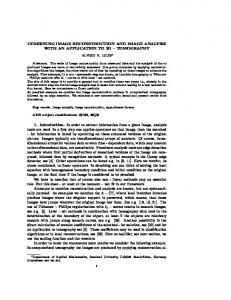
The first two terms on the right-hand side of (1) correspond to the intensities of the reference and object waves, respectively. In state-of-the-art digital holography systems, i(x) is recorded by a charge-coupled device (CCD) camera placed at the hologram plane [2, 4]. The adjective off-axis reflects the fact that the reference and object waves are separated by an angle θ, as shown in Figure 1. The off-axis arrangement has certain advantages, which will become clear when we address the reconstruction problem. 1.2. Hologram illumination We assume that the reference is a plane wave with a spatially2 2 constant intensity ir = |r(x)| . Let io (x) = |o(x)| denote the intensity of the object wave. To reconstruct the hologram, a plane wave u(x)—often referred to as the illumination wave—is used to illuminate the hologram. The resulting field ψo (x) = u(x)i(x) is given by ψo (x) =

ir u(x) + u(x)io (x) + u(x)r∗ (x)o(x) ! "# $ ! "# $ zero-order terms virtual image (2) + u(x)r(x)o∗ (x) . ! "# $ real image

The spatial locations of the various terms indicated above are shown in Figure 2. The zero-order terms comprise the plane wave ir u(x) and the object wave u(x)io (x), whose spatial variation is a function of the object. Since the reference and object-wave intensities modify the amplitude but not the phase of u(x), the zero-order terms propagate parallel to u(x). The spatial spread of the zero-order depends on the spectrum of the object wave. The virtual image is a reflection of the real image with respect to the hologram plane. The separation between the three images is precisely the advantage of the off-axis configuration. Note that for θ = 0◦ , it is not possible to spatially separate the various images. For the special case where u(x) = r(x), the real and virtual images are merely scaled by the intensity of the reference wave. When the distance of propagation equals the optical path distance d between the object and the hologram plane in the recording

0230.!""$

x Reference wave

x

z

z

Illumination wave

Zero-order term

θ θ

Hologram

θ

Object

Object wave

Hologram plane

Virtual image

Real image

Fig. 2: Off-axis digital holography—Reconstruction.

Fig. 1: Off-axis digital holography—Recording. area. Thus, the conventional reconstruction scheme is inefficient as far as utilizing the spatial resources is concerned. The standard approaches are based on estimating the object wave by spatial filtering [6]. This approach gives good results if θ is large enough to minimize the overlap between the object wave and the zero-order terms. Otherwise, the zero-order cannot be fully suppressed. In this paper, we propose a new technique to accurately estimate the complex object wave, despite overlap between the object wave and the zero-order terms. The technique is based on realistic assumptions about the recording conditions. The main advantage is that the technique fully suppresses the zero-order terms and therefore allows for efficient utilization of the available bandwidth. The organization of this paper is as follows. In Sec. 2, we analyze the spectral properties of the hologram. In Sec. 3, we develop the new reconstruction technique. The experimental results are provided in Sec. 4.

process, the real image comes into focus. In the existing methods for off-axis hologram reconstruction, the object wave is approximately recovered by using a bandpass filter [5, 6], an approach popularly known as spatial filtering. The estimated object wave is demodulated by removing the carrier frequency offset, or by using the complex conjugate component derived from a reference hologram [7], and then Fresnel-propagated numerically to adjust the focus of the reconstructed image. 1.3. Digital hologram reconstruction By employing the Fresnel approximation [1, 8], the underlying diffraction pattern can be specified up to second-order accuracy. In this framework, we have the following expression for the reconstructed wavefront: % & jπ 2 exp(j 2π d/λ) exp (ξ + η 2 ) ψi (ξ) = jλd λd ' % &( jπ 2 × F ψo (x) exp (x + y 2 ) , λd

2. SPECTRUM OF THE HOLOGRAM

where ξ = (ξ, η), λ is the wavelength and F denotes the Fourier transform operator. The reconstruction plane corresponds to x = ξ and y = η. The reconstructed wavefront is complex-valued and therefore can be decomposed into two parts—modulus and phase, which give rise to the amplitudeand phase-contrast images, respectively. The distance d is the adjustable parameter to bring the image into focus. In practice, due to the finite size of the hologram and due to sampling, the object wave, the twin image and the zeroorder have to be accommodated within a pre-specified region and without overlap among them. The twin image is redundant since it does not carry any more information than that already contained in the object wave; it is a natural consequence of the intensity measurement process and hence unavoidable. The zero-order component has a spread twice that of the object wave and occupies a major portion of the given

Consider the case where the reference is a plane wave; i.e., r(x) = A exp(−j #k, x$), where A is the complex amplitude, and the wave-vector is k = (kx , ky ), kx and ky being the wave-numbers in the x and y directions, respectively. The symbol #·, ·$ denotes the inner product of two index vectors and is defined in the usual sense; specifically, #k, x$ = kx x + ky y. Corresponding to this choice, (1) reduces to i(x) = |A exp(−j #k, x$) + o(x)|2 )2 ) 1 ) ) = |A|2 )1 + exp(j #k, x$)o(x) ) . A ! "# $ o(x)

o ˜(x)= r(x)

Note that multiplication by exp(j #k, x$) corresponds to a translation of the Fourier spectrum of o(x) to the location

!"!

Lemma 2. If o˜ ∈ (L1 ∩ L2 )(R × R) and F{˜ o} vanishes o| ≤ ) < 1, then outside Q1 = [0, +∞) × [0, +∞) and |˜ F{log(1 + o˜∗ )}(ω) also vanishes outside (−∞, 0] × (−∞, 0] almost everywhere.

−k. Consider the 2-D Fourier transform of i(x): * F{i}(ω) = |A|2 δ(ω) + F{o}(ω + k) + +F{o}(−ω − k) + q(ω) ,

Proof. The proof is similar to that of lemma 1.

where q(ω) denotes the 2-D autocorrelation of F{o}(ω), which gives rise to the object-wave zero-order term. In the special case where F{o}(ω) has a compact support [−σx , σx ] × [−σy , σy ], the autocorrelation also has compact support [−2σx , 2σx ] × [−2σy , 2σy ]. The problem is to exactly compute o from i but without the autocorrelation q. 3. PROPOSED RECONSTRUCTION TECHNIQUE The proposed method is based on the cepstrum [9], which is employed to suppress the autocorrelation. The main conditions required are that the object-wave modulation be confined to one quadrant of the frequency domain, and that the intensity of the reference wave be higher than that of the object. The key result is presented in the form of the following theorem. Theorem 1. If o˜ ∈ (L1 ∩ L2 )(R × R) has a Fourier transform F{˜ o} that is identically zero outside Q1 = [0, +∞) × [0, +∞) and |˜ o| ≤ ) < 1, then |1 + o˜(x)|2 specifies o˜(x) almost everywhere. Proof. We first need the following lemmas. Lemma 1. If o˜ ∈ (L1 ∩ L2 )(R × R) has a Fourier transform F{˜ o} that vanishes outside Q1 = [0, +∞) × [0, +∞) and |˜ o| ≤ ) < 1, then F{log(1 + o˜)}(ω) is also identically zero outside [0, +∞) × [0, +∞) almost everywhere. Proof. Since |˜ o| ≤ ) < 1, we invoke the Taylor series expansion for log(1 + o˜(x)): log(1 + o˜(x)) =

∞ , (−1)n−1 n o˜ (x). n n=1

(3)

Applying the Fourier transform operator F to (3), we get that F{log(1 + o˜)}(ω) =

∞ , (−1)n−1 F{˜ on }(ω). n n=1

(4)

Recall the convolution property of the Fourier transform: F{˜ on }(ω) = (F{˜ o} ∗ F {˜ o} ∗ F{˜ o} ∗ · · · ∗ F {˜ o})(ω). (5) ! "# $ n times

Since F{˜ o} vanishes outside Q1 , the right-hand side of (5) also vanishes outside Q1 almost everywhere. This property carries over to the right-hand side of (4).

!")

We continue with the proof of Theorem 1. Consider the o)+log(1+˜ o∗ ). Applying factorization: log |1+˜ o|2 = log(1+˜ the Fourier transform to both sides gives rise to the cepstrum: c(ω)

= F{log(1 + o˜)}(ω) + F{log(1 + o˜∗ )}(ω).

From lemmas 1 and 2, it follows that the functions F{log(1+ o˜)}(ω) and F{log(1 + o˜∗ )}(ω) have non-overlapping supports. By retaining the region corresponding to the support of F{˜ o}, we have that F{log(1 + o˜)}(ω) = F{log |1 + o˜|2 }(ω) · 1Q1 ,

(6)

where 1Q1 is the indicator function of the quadrant Q1 . The inverse Fourier transform of (6) gives log(1 + o˜(x)) = F −1 {F{log |1 + o˜|2 } · 1Q1 }(x), . ⇒ o˜(x) = exp F −1 {F{log |1 + o˜|2 } · 1Q1 } (x) − 1. (7) Equation (7) summarizes the proposed technique for complex object-wave reconstruction. The conditions on the spectral support and intensity can be satisfied by suitably adjusting the design parameters A, kx , and ky [2]. 4. EXPERIMENTAL RESULTS We next corroborate the theoretical findings with experimental results. The measurements are acquired in the transmission mode by using a digital holographic microscope with the objective having a magnification factor of 10 and a numerical aperture of 0.25. The specimen is a small collection of yew pollen grains in water. The specimen is illuminated with a coherent source of wavelength λ = 680 nm. The Fresnel distance at which the hologram is measured is d = 3.5 cm. An 8-bit CCD camera is used with spatial sampling steps of 6.45 µm in both the horizontal and vertical directions. The intensity ratio between the object and reference beams is controlled with a neutral density filter, which absorbs part of the power in the object beam, thus ensuring a stronger intensity of the reference. The (spatial) average reference-wave intensity is approximately 7 times higher than that of the object wave. The value is found to be a good compromise between the quality of reconstruction and the quantization of the interference fringes. The ratio can be increased provided that the measurements are finely quantized, thus potentially leading to an improvement in the overall quality of the reconstruction. The modulation is chosen to confine the imaging order in one

quadrant by changing the direction of propagation. For the conventional reconstruction, the Fresnel transform technique is used together with digital parametric phase masks for object-wave demodulation and the Fresnel integration technique for propagation. For more details of the hologram reconstruction, see [2, 8]. The hologram was also reconstructed using the cepstrum technique proposed in this paper. For a fair comparison, the reconstruction parameters for both spatial filtering and the cepstral techniques are kept the same, and one quadrant of the Fourier plane is filtered automatically in both cases. The results are shown in Figure 3. The zero-order term manifests as ghost artifacts in the amplitude image and as a high-frequency modulation in both the amplitude and phase images. Note that the artifacts are suppressed by the cepstral technique. From Figure 3(c) and (d), we see that the cepstral technique gives rise to better phase images than the linear technique and that the spatial extent is improved considerably. Although in principle the cepstral technique completely suppresses the zero-order, in practice, a small residue may be present because of the mismatch between the model and the practical scenario (for example, the assumption of a plane wave may not always hold) and inevitable measurement noise. 5. CONCLUSIONS We presented a new technique for zero-order-free image reconstruction in the context of digital holographic microscopy. Our technique is based on the cepstrum of the measurements and gives rise to exact results provided that some realistic conditions about the object-wave modulation and the relative intensities of the object wave and the reference are ensured. These conditions, however, can be easily realized in practice. We provided experimental results to support the theoretical calculations. The technique proposed in this paper may be extended to handle non-planar reference waves as well in order to increase the scope of its practical applicability. 6. REFERENCES [1] U. Schnars and W.P.O. J¨uptner, “Digital recording and numerical reconstruction of holograms,” Meas. Sci. Technol., vol. 13, no. 9, pp. 85–101, 2002. [2] E. Cuche, P. Marquet, and C. Depeursinge, “Simultaneous amplitude-contrast and quantitative phase-contrast microscopy by numerical reconstruction of Fresnel off-axis holograms,” Appl. Opt., vol. 38, no. 34, pp. 6994–7001, 1999. [3] U Schnars, “Direct phase determination in hologram interferometry with use of digitally recorded holograms,” J. Opt. Soc. Am. A, vol. 11, no. 7, pp. 2011–2015, 1994. [4] J. W. Goodman and R. W. Lawrence, “Digital image formation from electronically detected holograms,” Appl. Phys. Lett., vol. 11, no. 3, pp. 77–79, 1967.

!"(

E

F

Fig. 3: Amplitude (a-b) and phase images (c-d) corresponding to the linear reconstruction (a, c) and the cepstrum reconstruction (b, d); Specimen: yew pollen grains; the images (e) and (f) correspond to the black dashed boxes in (a) and (b), respectively. The scale bars are 20 µm long. [5] M. Takeda, H. Ina, and S. Kobayashi, “Fourier-transform method of fringe-pattern analysis for computer-based topography and interferometry,” J. Opt. Soc. Am., vol. 72, no. 1, pp. 156–160, 1982. [6] E. Cuche, P. Marquet, and C. Depeursinge, “Spatial filtering for zero-order and twin-image elimination in digital off–axis holography,” Appl. Opt., vol. 39, no. 23, pp. 4070–4075, 2000. [7] T. Colomb, J. K¨uhn, F. Charri`ere, C. Depeursinge, P. Marquet, and N. Aspert, “Total aberrations compensation in digital holographic microscopy with a reference conjugated hologram,” Optics Express, vol. 14, no. 10, pp. 4300–4306, 2006. [8] F. Montfort, F. Charri`ere, T. Colomb, E. Cuche, P. Marquet, and C. Depeursinge, “Purely numerical compensation for microscope objective phase curvature in digital holographic microscopy: Influence of digital phase mask position,” J. Opt. Soc. Am. A, vol. 23, no. 11, pp. 2944–2953, 2006. [9] A. C. Bovik, Handbook of Image and Video Processing, Academic Press, 2nd. edition, 2005.