Zero temperature parallel dynamics for infinite range spin glasses and .... steps if one starts with m (0) = 1. ... starting configuration m (t ) is the projection of the.
J.
Physique
48
(1987)
741-755
MAI
1987,
741
Classification Physics Abstracts 05.20
Zero temperature neural networks E. Gardner
(1),
parallel dynamics for infinite
B. Derrida
(2)
and P. Mottishaw
range
spin glasses
and
(2)
(1) Department of Physics, University of Edinburgh, Edinburgh EH9, 3JZ, U.K. (2) Service de Physique Théorique, CEN Saclay, 91191 Gif-sur-Yvette Cedex, France (Reçu
le 5 novembre 1986,
accept6
le 20
janvier 1987)
Nous présentons les résultats de calculs analytiques et numériques pour une dynamique parallèle à Résumé. température nulle de modèles de verres de spin et de réseaux de neurones. Nous utilisons une approche analytique pour calculer l’aimantation et les recouvrements après quelques pas de temps. Dans la limite des temps longs, cette approche analytique devient trop compliquée et nous utilisons des méthodes numériques. Pour le modèle de Sherrington-Kirkpatrick, nous mesurons l’aimantation rémanente et les recouvrements à des temps différents et nous observons des décroissances en loi de puissance. Quand on itère deux configurations différentes, leur distance d(~) au bout d’un temps infini dépend de leur distance initiale d(0). Nos résultats numériques suggèrent que d(~) a une limite finie quand d(0) ~ 0. Ce résultat signifie qu’il y a un effet collectif entre un nombre infini de spins. Pour le modèle de Little-Hopfield, nous calculons l’évolution temporelle du recouvrement avec une pattern mémorisée. Nous observons un régime pour lequel le système retient mieux après quelques pas de temps que dans la limite des temps longs. 2014
We present the results of analytical and numerical calculations for the zero temperature parallel dynamics of spin glass and neural network models. We use an analytical approach to calculate the magnetization and the overlaps after a few time steps. For the long time behaviour, the analytical approach becomes too complicated and we use numerical simulations. For the Sherrington-Kirkpatrick model, we measure the remanent magnetization and the overlaps at different times and we observe power law decays towards the infinite time limit. When one iterates two configurations in parallel, their distance d(~) in the limit of infinite time depends on their initial distance d(0). Our numerical results suggest that d(~) has a finite limit when d(0) ~ 0. This result can be regarded as a collective effect between an infinite number of spins. For the Little-Hopfield model, we compute the time evolution of the overlap with a stored pattern. We find regimes for which the system learns better after a few time steps than in the infinite time limit. Abstract.
2014
1. Introduction.
Zero temperature dynamics have become of more and more interest in the study of spin glasses and of neural networks [1-5, 9, 10, 19]. They exhibit qualitatively the same features (many metastable states, remanence effects) as spin glasses at low temperature. However they are much simpler to study from a theoretical point of view because the effect of thermal noise is eliminated. They may also have practical advantages if one wants to build pattern recognition devices. The reason that zero temperature dynamics are non-trivial and interesting is the existence of many metastable states [6]. These metastable states are responsible for remanence effects [7], very slow relaxations and sensitivity to initial conditions.
They are also at the origin of all optimization problems [8]. At the moment one knows, at least in infinite ranged models, how to compute the number of metastable states [6, 11]. However much less is known about the sizes and the shapes of their basins of attraction which play a crucial role in zero temperature dynamics [3, 11, 12]. Even the characterization of these sizes and shapes is not easy. present work, we will develop an approach temperature dynamics. This paper will treat
In the to zero
it simplifies our calculations but we think that some of our results could be generalized to serial dynamics. We will mainly consider a system of N Ising spins. (a i = ± I ) with interactions, Ji, , between all pairs of distinct spins. The interactions are defined such that
only parallel dynamics because
Article published online by EDP Sciences and available at http://dx.doi.org/10.1051/jphys:01987004805074100
742
and Jii 0, but more general cases can be same analytic approach. the dealt with using that the configurations at means Parallel dynamics time step t is given by the rule
Jl
=
Jji’
=
after an arbitrary number of time steps, in practice the number of order parameters increases very quickly with time and makes each time step more difficult. In section 3, we apply the same method to the two neural network models. We give the analytic expression of the overlap with a stored pattern after one and two time steps. In section 4 we present various numerical calculations for the SK and the Little-Hopfield models with
where all the spins are updated at the same time. We consider, the 7 are random variables which remain fixed in time. Therefore for a given sample, and a parallel zero temperature dynamics. at time t For the SK model at short times the numerical 0, the given initial configuration results at detertime t is later any uniquely agree with the results obtained by the analytic configuration method of section 2. At longer times, these results mined by iterating equation (1.1). We will consider three models. Firstly, the Sher- indicate a power law decrease of magnetization and rington-Kirkpatrick [13] spin glass model for which of the overlap between successive times. The study the Ji are independent random variables with a of the overlap between two configurations show that the basins of attraction of the different valleys have a distribution high degree of interpenetration. For the Little-Hopfield model, we obtain the projection on a stored pattern after one, two and an infinite number of times steps as a function of the Secondly, the Little-Hopfield model [14, 15] which is projection at time t 0. Again the results at short a pattern recognition model. The Jij are given in this times agree with the results of section 3 whereas the model by results at long time show a clear change between the good recall and the bad recall phases.
{u?}
=
=
where Na is the number of patterns which are stored is the value of spin ai in the
and lJ.L) = :t 1
pattern
The map, equation (1.1), is deterministic, so that at t 0, given an initial spin the spin configuration, at any later time, t, is uniquely determined. Consider
configuration {ulO)}
tk.
The third model we consider is a generalization of the Little-Hopfield model to the case of p-spin interactions [16]. The updating rule, equation (1.1), is generalized to
where
=
{uf},
where
and the number of patterns is 2 NP -’ In section 2 we present an analytic approach which allows one to compute the time evolution of magnetization, overlaps, local fields, etc. averaged over disorder, after an arbitrary number of time steps. For the SK model we compute certain quantities exactly up to the 5th time step. Although the method can in principle be used to compute all properties
a lp! .
Where ( ) /y B
2. The SK model.
denotes
an
average
over
f o-
is the descendent of is unity if after T iterations of the map and zero otherwise. The disorder average of the probability that for a randomly chosen sample, is the descendent after T time steps. This allows, for example, the average magnetization after T time steps from an initial configuration to be written This
quantity
{ u ?}
{o-}
{ u?}
the random
couplings.
nT( {cr,9), {ul}) is
of ( at)
743
As
will show in this section the natural
we
parameters of the problem are related to the disorder correlation functions between the and the local fields Hi’ given by
averaged
cr!,
so
spins,
computed
from the
following generating functional,
that
and
y(O, 0) = 1, since for a given initial configuration, the configuration at each later time is uniquely determined. From equation (2.3), y (g, h ) Note that
is
at different times. These can be
invariant
under
the
gauge transformation Jij Ji si 8j’ crf --+ Ei uf (and therefore Hj - Ei Hf) for all time t > 0. This transformation changes the initial configuration from o-° to E at, so that y (h, g ) is independent of the initial configuration. For convenience we shall take a normalized trace (Tr 1=1) over the initial configuration. Of particular interest is the average magnetization after t time steps, from an initial configuration with all spins up. --+
m (t ), given by (2.5) is the magnetization after t time steps if one starts with m (0) = 1. For any other starting configuration m (t ) is the projection of the configuration at time t on the configuration at time 0. If one starts at t 0 with a configuration with then at time t, the magnetization tk, magnetization will be J.Lm (t). In order to perform the averages over the random couplings Jij, we will use the following integral representation of the 0 functions, in equation (2.3), =
Thus
where,
where
Performing
Retaining
the disorder average,
terms of
leading -
over
the distribution
p (Jij) equation (1.2) gives
order in N, in the exponent, this r
can
be written
744
The first term in the exponent constraint
can
be reduced to
Similarly the second term in the exponent of identities. The result is
a
single
sum over
equation (2.10)
can
sites
be
by introducing
decoupled using
the delta function
Gaussian
integral
where the Const. depends only on N and J and plays no role in the following because we use a saddle calculation. Thus y(h, g), equation (2.7), can be written as an integral over the variables r, t s tlt2; which can be computed by steepest descents in the limit N - oo.
point
ptl ’2, qtl t2,
where
and
In all the sums the upper limit is T’ and the lower limit is 1. The saddle point equations are for 9 ( t i, t j) 0 and h(ti,tj) = 0 =
745
where the
with
expectation value h(tl, t2) 0 and g(tl, t2) =
( is with respect to the =
0,
A useful check on the saddle point equations, is that in zero field the exponent in (2.13a) should vanish as y(0, 0 ) = 1 from equation (2.3). A direct evaluation of these expectation values in zero field (h y 0), (see Appendix 1 for details) show that a number of order parameters vanish: =
generalized
trace defined in
equation (2.13c),
i.e. with
=
We will
consider the time evolution of the
after t time steps
If
The physical meaning of the order parameters can be obtained by taking derivatives of equation (2.13a) with respect to h (tl, t2 ) and g (tl, t2 ) and comparing with equations (2.4). The derivative with respect to h gives
now
magnetization starting from an initial configuration with magnetization 1. Setting tl = 1 in equation (2.16) gives for the average magnetization average
know the properties of the system at it is that one does not need to know clear time t, what happens at later times t’ > t. Therefore the order parameters defined at a particular pair of time steps can depend only on parameters defined at previous time steps. Thus at short times the properties of the model are determined by a few order parameters. At successive time steps the number of order parameters increases rapidly (approximately as the square of the time). The equations obtained from the saddle point for the remanent magnetization after two times steps one wants to
are
q t’ t2
q t’ t2
is evaluated in zero field. Thus is equal to the overlap between configurations at time t1 2013 1 and t2 - 1- If one makes the global change {Jij} --+ - Jij), the dynamics (1.1) of the spins implies that aj - - aj for odd t and aj - aj for even t. Therefore since the distribution of 7 is one has symmetric,
where
true for all times t1 and t2 with we did not find how to derive it but 1 t1 - t21[ odd, from the saddle point equations. easily Taking the derivative of equation (2.14b) with
This is
certainly
respect to g, gives
tl1 and equations (2.15) have been used. Due to the symmetric distribution of the Jij’s, the left hand side of equation (2.17) vanishes when 1 t1 t21[ is even, so that
where t2
-
where
The equations for the order parameters and magnetization upto T 4 are given in appendix 2. Using equations (2.21), (2.16), (2.18) and the results of appendix 2 we obtain for the first few order parameters, =
746
since m (t ) vanishes for odd values of t the magnetization oscillates between zero and a finite value which decreases with time. Clearly its value at successive time steps provides one way of approximating the final remanent magnetization. Numerical results to be described in section 4 show that the final value is 0.23 ± 0.02 so the approximate value m(4) 0.468 is still rather far from the correct one.
We consider spin configurations which overlap with one of the patterns, and a microscopic overlap (of order N - 1/2) with the remaining patterns. The overlap between a given and the spin at pattern time t is defined by
orthogonal. have
a
finite
{/ II)}
configuration {u f}
=
m’
3. Neural network models.
The time evolution of depends strongly on the choice of the initial spin configuration at t 0. Here we shall choose the initial spin configuration to have a finite overlap with the a = 1 pattern, and a microscopic overlap with the remaining patterns. We assume that this property holds for the subsequent spin configuration in time. This assumption is shown to be self consistent, at least for short times. A generating functional for the average spin-spin correlation function can be defined in the same way as for the SK model : =
In this section
show how the
of the
properties equation (1.3), and its p-spin generalization, equations (1.4), (1.5) can be obtained analytically. The method is similar to that used for Little
we
model,
the SK model in section 2. In the Little-Hopfield model N a patterns are chosen at random, thus the overlap between two patterns is typically of order N - 1/2. In the N -+ 00 limit this overlap is zero and the patterns are
where ) {Î} configuration
indicates
an
average
over
all the N a patterns. The trace, Tr’
the initial
spin
is restricted to
so that it has overlap 2 g -1 with for the 0-functions, y becomes
the tk = 1 pattern. Introducing the integral representation, equation (2.6),
I
In order to
so
over
so Ui
perform
that y becomes,
the average
over
the patterns
we use
the
identity
747
where
Using
assumption that the spin configuration has a finite overlap only with pattern 1, only the first expansion of In cos [ ] contributes to leading order in N. Thus Y(xl!, crl!, g’ , n) becomes
the
term in the
·
The
sums on
sites and
The final form for
where
and
and
y (hrl t2 )
sums on
is then
patterns
can
be
decoupled by using
the identities
748
The integral in equation (3.9a) can now be computed in the limit N -+ oo by steepest descents. The saddle
point equations
are
the spin configurations and the patterns with A >. 1. Using the results, equation (3.12), and an argument similar to that given in appendix 1, we find
computed the parameters for the first step ( T 2). Note that the initial overlap
We have two time
is
=
mr = 2 g - 1,
equation (3.3). one
time step
The
new non-zero
steps
where the to the
expectation value ( ) 2 ±is weight in equation (3.9d), and
it must from the constraint The non-zero order parameters after as
are
order parameters after two time
are
with respect
where the expectation value > w is with respect to the weight inequation (3.9c). The parameters in equation (3.10) are related to correlation functions involving local fields and spins in similar way to the SK parameters in section 2. All the correlation functions are of course always real but due to our definition of the order parameters in the present section some order parameters are imaginary. Using a similar argument to that of appendix 1 we find that certain order parameters are zero :
The qualitative behaviour of the overlap ml 1 with a stored pattern after one time step (Eq. (3.14)) is different depending on whether a, is greater than or less than 2/7T :::L-. 0.64 ; for a greater than this value ml is always less than whereas for a 0:0, there is a fixed point of equation (2.14) at m mo (a) m decreases if m :::. mo (a) and increases if m mo (a ). The transition at a o is second order since mo (a) --+ 0 as a -+ a 0. Similarly, equation (3.15) implies that mf increases after the is sufficiently second time step if its starting value small and if a 0.67. Physically, this means that the system goes towards a learned pattern after one (two) time steps provided a 0.64 (0.67). These values of a are much larger than the value suggested by thermodynamic calculations [9, 20] which predict the existence of an energy valley correlated with the input pattern only if a ac - 0.14. The transition at ac is first order ; m jumps from zero for a > a c to a non-zero value. However the a c predicted by thermodynamic
ao
=
mo
m°
-
The
non-zero
parameters have the following physical
interpretation ; q tl t2 is the overlap between spin configuration at time t1 2013 1 and t2 - 1 ; stl t2 is related to the overlap of local fields and spins (cf. Eq. (2.18)) and ml is the overlap between pattern 1 and the spin configuration at time t. The parameters in equation (3.11) are related to the average of the products of the overlaps between
749
calculations may not be relevant to dynamics. Moreover, we will see in section 4 that the critical a for parallel dynamics in the long time limit is clearly smaller than 0.67.
The calculations for multiconnected neural network model can be done in a similar way to the calculations for the Little-Hopfield model. The analogue of equation (3.4) is for htt t2 0,
The p spin calculations however turn out to be simpler than the two-spin calculations because correlations between different Ji1 ... arise only from the of the interactions symmetry [16]. The reason is as
follows ; equation (3.16) includes a product over microscopic patterns of exponential factors. If each
The second order term may be
exponentiated
=
of these
exponentials
is
expanded and the average performed the linear
at each site is
over
patterns
term
vanishes and
and 5-functions introduced to
give
where
where,
All terms of
expansion P
over
higher order than the microscopic patterns
second in the are of order
N 2
relative to the second order term and therefore do not contribute in the thermodynamic limit. For p 2 the whole series can be resumed to give the determinant W (q, s, p ) of equation (3.9c). The equation for ml after the first time step is then, =
Little model (3.14) the fixed point of the first stage of parallel interaction of the multiconnected model (3.19) are identical to the replica symmetric solution for the metastable state close to the pattern in the thermodynamic calculation [16]. There are two fixed points for a a,, (p ) which approach one another as a - a c (p ) and the transition at a c is first order. 4. Numerical
In contrast to the
corresponding equation
for the
study of long time behaviour.
In this section, we will first present numerical results obtained for the zero temperature parallel dynamics of the SK model. The calculations were done on
750
samples of N sites (25 -- N , 400 ) and the in (4.1) gives q ’ ’ l,’- 1 defined by (2.16) in the limit quantities were averaged over 1 000 to 2 000 samp- N -+ 00. les. The interactions Iii were randomly chosen The remanent magnetization according to a flat probability p (Iii) (p (Jij) = 1/2 Jo forI JijI -- Jo and p (Iii) 0 forI IiiI >. JO). In the thermodynamic limit, all symmetric distributions of give the results which depend only on depends strongly on the size N (Fig. 1) whereas at Iii for short times, the size dependence of mN (t ) is much (IÕ) the SK model. In table I, we give numerical results obtained for weaker. This makes the analysis of the long time the magnetization m(2), m(4) and m(oo) at times behaviour of the magnetization rather difficult. The t 2, t 4 and t = oo and for the overlap q 42 and following two attempts were made : q53. All these quantities except m(oo), describe the system after a few time steps and can be compared with the analytical results of section 2. We see that finite
=
=
=
the agreement is excellent. One can also see in table I that the long time properties (like m(oo)) depend much more on the size N than the short time
properties. In the approach developed in section 2,
the calculations become more and more tedious as one increases the number of time steps. This makes the understanding of the long time behaviour quite difficult by this analytic approach. So for the long time behaviour, we could only use the numerical simulations. We have computed the magnetization mN (t ) at the t-th time step (starting at t 0 with mN (0 ) = 1) and the correlation qN (t, t - 2) between the configurations at time t and at time t 2 for samples of N spins. Due to gauge invariance, q t, ’ -2 is independent of the starting configuration when it is averaged over disorder. =
-
We did not consider q (t, t 2013 1) as it vanishes at all times equation (2.17). This is because for each i and t, u i (t) U i (t - 1) is an odd function of the interactions Iij. One should notice that qN(t, t - 2 ) defined
Fig.
1.
versus
The magnetization MN (00 ) of the SK model N - 1/2. Extrapolating to N -+ oo gives moo ( 00 ) = -
0.23 ± 0.02.
Table I. Magnetization at times 2, 4 and oo and the overlaps qt,t- 2 for t 4 and 5 for the SK model. The results at short time converge quickly to the predictions of section 2. The convergence of m(oo) is much slower. -
=
751
First, if one considers MN size N, the results seem to long times
(t) - MN (00 )
for each
decay exponentially
at
Our numerical results suggest that TN increases like 0.5. An accurate determination of a N" where a is not easy because we can only increase N up to a few hundreds and TN has to be extracted from the long time behaviour (t::’ T N ) for which the error bars are the biggest. On the other hand, if we try to look at M. (t) - m. (oo ), one finds a power law =
The estimation of i3 is not easy either, because one needs to take the limit N -+ oo. For short times t, this is not very hard because mN (t ) does not vary much with N but for t -+ oo, this is more difficult (see Table I and Fig. 1). Also the range of times on which the power law (3.3) can be observed is rather limited 1 -- t , 20 because our sizes N are small and (3.3) only be valid for t -,- T N. However a log-log plot gives 0.5 -- -- 0.7 depending on what we choose for MN (00 versus N - 112. The convergence to N -+ oo is rather slow and our estimate for m. (oo ) is
Fig. 2. - 1 - q+ 1, t -1 versus t. The overlap q+ 1, t -1 is the overlap between a configuration at time t and at time t 2. We see that 1- q+ 1, t -1 decreases like t-312 over a -
range of times which increases with N.
and
a
long time regime which is size dependent.
The
exponent 3/2 is rather accurately determined. In figure 2 we see that, the range on which (4.5) holds The N - 1/2 convergence is the same as the one found by Kinzel for serial dynamics [7]. This value differs from moo (oo ) 0. 14 -t 0.01 predicted by Kinzel for sequential dynamics. This difference is not surprising because the two dynamics have no reason to give the same remanent magnetization. For example for 1d =
spin glasses, sequential dynamics give m.(oo) = 1/3 (see Ref. [12] and references therein) whereas parallel dynamics would give m.(oo) 2/3. Also a value of j3 0.5 (see Eq. (3.3)) is rather similar to what had been previously found or predicted for finite temperature dynamics near the spin glass transition (Ref. [18] and references therein). It is not =
=
clear however whether our value of j8 could be compared with any result even at low temperature because one expects that moo ( 00 ) =1= 0 for T = 0 whereas m.(oo) 0 at low temperature. The long time behaviour is much easier to study when one considers the time evolution of qn(t,t -2). In the limit t-+ oo, qN(t,t-2)-+ 1 independent of N. So the problem we had because of the N-dependence of the remanent magnetization is not present here. In figure 2 we show log (1 - qN (t, t - 2 ) ) versus log t for N = 100 and 400. We see for each size two regimes. The N short time regime where =
=
increases with N and therefore (4.5) is probably valid at all times in the thermodynamic limit. The result (4.5) is compatible with the power law (4.3) 0.7 since one has always and the estimate 0.5 , /3 I
(3.6) expresses that the change in the magnetization is always less or equal to the number of spins which have flipped. Another quantity which can be computed at short times analytically and at long times numerically is the overlap between two configurations. If one chooses 2 configurations (ai(0)) and (Ti(0)) at time t 0, and if both configurations evolve according to the same set of interactions Jij one can try to compute the time evolution of the overlap Q (t) =
At short times, calculations very similar to those presented in section 2 give
752
where
size N, it is rather clear that when d (0 ) vanishes
We see from these expressions that the calculation becomes more and more difficult as one increases the number of time steps and so here again, we could only study the long time behaviour by means of numerical simulations. In figure 3 we show d(oo ) versus d (0 ) for 0 , d (0 ) _ 0.05 where d (t ) is the
d (oo )
does not vanish
It is not very easy to determine the limiting value accurately because one needs to take two limits, Q (0) -+ 1 and N -+ oo. However, the fact that d ( oo ) does not vanish if d(0) -+ 0 gives an idea of the ’ structure of the basins of attraction of the attractors. Two starting configurations even if they are very close will evolve to attractors which are far
apart. This means that the frontiers, between basins of attraction are dense in phase space. Also this means that there is a cooperative effect between an infinite number of spins : if the dynamics could be reduced to finite clusters of spins, then when d(0) -+ 0, the number of clusters for which the configurations ai(O) and Ti(O) differ would be proportional to d(O). Only these clusters could contribute to d(oo ) and therefore one would have d(oo ) proportional to d(0). The fact that d ( (0) does not vanish as d (oo ) -+ 0 means that there is a cooperative effect involving an infinite number of spins. The same results has already been found in the dynamics of other random systems : random networks of automata
[17].
For the Little-Hopfield model, we have computed the overlap m’ with a stored pattern as a function of for several values of a. In figures 4, 5 and 6 we show our results for a 0.1, a 0.4 and a 0.9. For all these values of a, we observed that ml has a limit mf as t -+ oo. This means that the oscillations of mi between odd and even times (which are present in the SK model) are either absent or too small to be observed (i.e. smaller than our error bar) for these values of a. We see that for a 0.1 (Fig. 4), the system remembers (since for one finds mi very close to 1). It is interesting to notice that mf is not always a monotonic function of time. For a 0.4, the system does not remember in the limit t -+ oo (mi However for short times, we see that there is a range for which and This means that larger than the configuration in the first time steps goes towards the pattern but at later times goes away. Lastly for a and the configur0.9, we have always mf ation always evolves away from the pattern.
m°
=
=
=
=
mo:::. 0.5,
and d(aJ ) at time t = 1, t versus the initial distance d (0) between two configurations for the SK model. The two curves are the result of equations (4.8)-(4.11). We see that d (oo ) does not seem to vanish when d (0) -+ 0.
Fig.
3.
-
=
The distances 2 and t = oo
d (1 ), d(2)
distance between the two defined by
We
see
that,
even
d(oo )
still
configurations
and is
depends on the system
=
m°).
ml
=
ml are
m°.
: mr
There is therefore a qualitative difference between the results at long times and those for the first few time steps. For a 0.64 (0.67), the system remembers after 1 (2) time steps whereas at large time, the system remembers only if the initial overlap is
753
sufficiently large. This suggests a way of improving dynamics for a below 0.64 (0.67). Since nonequilibrium states which do not appear in the thermodynamic calculations exist for values of a above as well as below a [11] it might be possible after a few time steps of parallel iteration to define a way of annealing into a metastable state closer to the the
pattern. We have not observed 2-cycles for values of 1. However, in the limit a - oo, iterations from a pattern is equivalent to iteration from any initial configuration ; for example equations (3.14), (3.15) reduce to those of the SK model (2.17), (2.21) ; and in this case the remanent magnetization is zero at odd times and non-zero at even times. Therefore either there exists a finite value of a > 0.9 above which limit cycles appear or the oscillation of mt are present at all values of a but are too small for a 0.9 to be observed with our error bars. a
Acknowledgments. 4.
The
overlap mi
for t = 1, 2 and oo with a stored : a 0.1 (Fig. 4a), a 0.4 (Fig. 4b), a 0.9 (Fig. 4c). The points are the results of numerical simulations and the curves were obtained from equations (3.14) and (3.15). For a 0.1 (Fig. 4a), the system learns. For a 0.4, the system goes towards the pattern for the first time steps if m° is small enough but does not learn in the long time limit (the dashed straight line is m’ m?). For a 0.9 (Fig. 4c) the system does not learn even in the finite time steps.
Fig.
-
pattern =
versus
mo for the Little model
=
=
=
=
=
=
E. G. would like to thank the Service de Physique for their hospitality whilst visiting Saclay. Financial support for E. G. was from the Science and Engineering Research Council, U.K. and for P. M. from the Royal Society. Part of the work was done while B.D. was visiting the Institute of Theoretical Physics at Santa Barbara and was supported by the U.S. National Science Foundation under grant N° PHY 82-17853 supplemented by funds from the U.S. National Aeronautics and Space Adminis-
Theorique
tration.
754
Appendix
1.
In this appendix we show that any expectation value with respect to y, equations (2.13c), of the form
in zero field where S (xt, U t) depends only on times earlier than T. This expectation value contains a term of the form
Note that C (x,, a,) does not depend cr T. Taking the trace on u T gives
on
XT
or
In the second term make the change of variable : XT-+-XT; ’AT-+- A T, so that
where
Thus the
expectation value, (A.I),
is
zero :
Appendix 2. In this appendix we give the results for the order parameters and magnetization up to 4 time steps, obtained from the saddle point equation (2.14a) for the SK model. The results up to t 2 are given in equation the are : ones (2.21), remaining =
755
and
where erf
using
the formula,
where
References
[1] BIENENSTOCK, E., FOGELMAN-SOULIÉ, F. and WEISBUCH, G., Disordered Systems and Biological Organisation (Springer Verlag, Heidelberg) 1986.
[2] PARGA, N. and PARISI, G., preprint 85. [3] KANTER, I., SOMPOLINSKY, H., preprint 86. [4] WEISBUCH, G. and FOGELMAN-SOULIÉ, F., J. Physique Lett. 46 (1985) L-623. [5] FOGELMAN-SOULIÉ, F., GOLES-CHACC, E. and PELLEGRIN, D., Discrete Applied Math. 1984. [6] TANAKA, F. and EDWARDS, S.F., J. Phys. F 10 (1980) 2471.
DOMINICIS, C., GABAY, M., GAREL, T. and ORLAND, H., J. Physique 41 (1980) 923. BRAY, A. J. and MOORE, M. A., J. Phys. C 14 (1981) 1313, C 13 (1980) L469. W., Phys. Rev. B 33 (1986) 5086. KINZEL, [7] [8] KIRKPATRICK, S., GELATT, C. D. and VECCI, M. P., DE
Science 220
(1983)
671.
[9] AMIT, D. J., GUTFREUND, H. and SOMPOLINSKY,
H., Phys. Rev. A 32 (1985) 1007 ; Phys. Rev. Lett. 55 (1985) 1530. A. D., GARDNER, E. J. and WALLACE, D. J., J. Phys. A 20 to appear. [11] GARDNER, E., J. Phys. A 19 (1986) L1047. [12] DERRIDA, B. and GARDNER, E., J. Physique 47 (1986) 959. D. and KIRKPATRICK, S., Phys. Rev. SHERRINGTON, [13] Lett. 32 (1975) 1792. [14] LITTLE, W. A., Math. Biosc. 19 (1974) 101. [15] HOPFIELD, J. J., Proc. Math. Acad. Sci. 79 (1982) 2554. [16] GARDNER, E.,J. Phys. A 20 to appear. Lett. 1 [17] DERRIDA, B. and POMEAU, Y., (1986) 45. [18] SOMPOLINSKY, H. and ZIPPELIUS, A., Phys. Rev. Lett. 47 (1981) 359. [19] PERETTO, P., Biol. Cybernet. 50 (1984) 51. [20] FONTANARI, J. F. and KÖBERLE, R., São Carlos preprint (1986).
[10] BRUCE,
Europhys.