zigbee-based intra-car wireless sensor networks: a case study

TONGUZ LAYOUT

12/4/07

4:13 PM

Page 67

WIRELESS SENSOR NETWORKING

ZIGBEE-BASED INTRA-CAR WIRELESS SENSOR NETWORKS: A CASE STUDY HSIN-MU TSAI AND OZAN K. TONGUZ, CARNEGIE MELLON UNIVERSITY CEM SARAYDAR, TIMOTHY TALTY, MICHAEL AMES, AND ANDREW MACDONALD, GENERAL MOTORS CORPORATION

ABSTRACT

Engine compartment

Front B

6

0 1

avilion N5495 laptop

Parser/logger to record the packets received by BS

The authors report the results of a ZigBee-based case study conducted in a vehicle. Overall, the results of the experiments and measurements show that ZigBee is a viable and promising technology for implementing an intra-car wireless sensor network.

There is a growing interest in eliminating the wires connecting sensors to the microprocessors in cars due to an increasing number of sensors deployed in modern cars. One option for implementing an intra-car wireless sensor network is the use of ZigBee technology. In this article we report the results of a ZigBee-based case study conducted in a vehicle. Overall, the results of the experiments and measurements show that ZigBee is a viable and promising technology for implementing an intra-car wireless sensor network.

INTRODUCTION Wireless sensor networks have been implemented in various monitoring applications such as industrial, health, environmental, and security. Recently, vehicular applications have entered the list due to several important considerations. As the number of sensors used in modern cars keeps increasing, the cost and weight associated with their integration also increase. If the wires can be replaced with a suitable wireless technology, sensors can communicate with the control unit (microprocessor) in a wireless fashion. It is anticipated that such a solution could lead to significant benefits in reducing cost, providing an open sensor network architecture that will be scalable as the number of sensors keep increasing, and reducing the weight of the car, which will enhance fuel efficiency. While several wireless technology options seem plausible, it is not clear what the optimum choice is. To this end, in this article we report a case study using wireless sensor nodes that are compliant with ZigBee. In this article we aim to answer the following questions: • Is ZigBee technology a promising/viable technology for building an intra-car wireless sensor network? • What are its strengths and weaknesses compared to other alternatives such as radio frequency identification (RFID)?

IEEE Wireless Communications • December 2007

• How easy is it to build an intra-car sensor network based on currently available off-the-shelf ZigBee sensor nodes? ZigBee is an industry alliance that promotes a set of rules which builds on top of the IEEE 802.15.4 standards [1]. It is clear that the feasibility of any communication technology for an intra-car wireless sensor network has to be examined in a bottom-up fashion, starting from the physical (PHY) layer. The communication between sensor nodes and a base station in the car will depend on several factors, such as the power loss, coherence bandwidth, and coherence time of the underlying communication channels between the sensor nodes and the base station. In this article channel behavior under various scenarios is observed for ZigBee nodes placed throughout a midsize sedan.In general, our experiments and measured results indicate that ZigBee is a viable and promising technology for implementing an intra-car wireless sensor network. To the best of our knowledge, this article presents the first attempt to characterize ZigBee performance within a vehicle environment. The rest of the article is organized as follows. First, the details of the experimental setup are described. Then the results of the experiments and discussion of these results are presented. We then propose a set of detection algorithms and an adaptive strategy that can adjust to channel conditions for improving the error performance of the wireless channel, and preliminary evaluation results are presented. Subsequently, we present a discussion on the feasibility of using ZigBee technology for building a wireless sensor network in a car. Finally, concluding remarks are given.

EXPERIMENTAL METHOD SENSOR NODE HARDWARE In our experiments we use Crossbow MPR2400 [2] as our sensor node hardware platform. The specifications are shown in Table 1.

1536-1284/07/$20.00 © 2007 IEEE

67

TONGUZ LAYOUT

12/4/07

4:13 PM

Page 68

Parameter

Value/description

Processor

ATMega 128L processor

Radio chip

Chipcon CC2420 radio

Operating frequency

2.4 GHz

Effective data rate

250 kb/s

Modulation format

Offset quadrature phase shift keying (OQPSK)

■ Table 1. Crossbow MPR2400 (MICAz) specification.

EXPERIMENTAL SETUP AND SENSOR NODE FIRMWARE Figure 1 shows the experimental setup. In the experiment, sensor nodes (SNs) are placed in different locations in the vehicle. The base station (BS) is placed inside the instrument panel of the vehicle, next to the vent. The BS is connected to an MIB510 programmer, and an RS232-to-USB converter is used to connect the laptop and MIB510. The following describes the functionalities of the BS and SNs used in our experiments. Base station: • Collect the sensor packets sent by the sensor nodes and relay those packets to their destinations. In the experiments the packets are relayed to the connected laptop. In a realworld in-car wireless sensor network, the packets are relayed to the corresponding con-

trol unit. In this aspect the BS has functionality similar to that of the ZigBee coordinator specified in the ZigBee specification [1].1 • Log various metrics such as received signal strength indicator (RSSI), link quality indicator (LQI), and cyclic redundancy check (CRC) of the received packets. • In our experiments the BS also relays the control message from the laptop to the SNs. • In the real implementation, the BS could also execute detection algorithms and issue commands to the SNs in order to improve the link quality. Sensor node: • Periodically retrieve sensor information from the attached sensors and send (broadcast) sensor packets to the BS. In the experiment the packet logger/parser software in the laptop processes the packets relayed by the BS, and saves them to a log file for further analysis. The command sender in the laptop can be used to issue commands to adjust the parameters of SNs such as transmitting power and packet sending rate. The firmware of sensor nodes and the base station is based on TinyOS 1.1.15 [3]. TinyOS is an open source component-based operating system and a platform targeting wireless sensor networks. Our implementations use various application programming interfaces (APIs) and libraries provided by TinyOS.

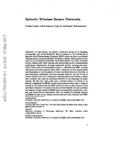
SENSOR NODE LOCATIONS The vehicle used in the experiment is a General Motors 2005 Cadillac STS. Figure 2 and Table 2 show the locations of the SNs as well as the BS in the vehicle.

Sensor pkts

Base station

Sensor node

BS firmware SN firmware Log metrics Log sensor data

Relay CMDs CMD packet

TinyOS 1.1.15

MIB510 programmer

TinyOS 1.1.15

MTS101 sensor board RS-232->USB

CMD packet

Sensor pkts

Light, temperature, or air quality sensors

Sensor

Serial forwarder

1

However, most of the functionality of the ZigBee coordinator is not implemented in our experiment (e.g., security and network layer functionalities) since the main objective is to evaluate the PHY layer performance of the ZigBee sensor node.

68

Legend

CMD sender Packet logger/parser

Sensor monitor

Hardware Vendor software

HP Pavilion N5495 laptop

Implemented/modified software

■ Figure 1. Block diagram of the experimental setup.

IEEE Wireless Communications • December 2007

TONGUZ LAYOUT

12/4/07

4:13 PM

Page 69

EXPERIMENTAL SCENARIOS We performed different experiments under various scenarios shown in Table 3. The details of these scenarios are discussed in the following.2 Location: •Maintenance garage. This is similar to the service depot of a regular car dealer. Technicians walk by frequently, and several other cars are parked nearby. There is a lot of service equipment in the garage. •Corporate parking lot. This is a regular corporate parking lot. The test vehicle was parked in one parking space and surrounded by other cars. Pedestrians occasionally passed by the test vehicle. Nearby vehicles sometimes moved in or out of the parking lot. •Road. This is the driving scenario. The car was driven on the highway most of the time and sometimes on large (multi-lane) local roads. Driver: In the “driver present” scenarios the driver was sitting in the car and had frequent movements, such as operating the A/C, radio, and steering wheel. In the “driver not present” scenarios the driver’s seat was empty. Engine: In the “engine on” scenarios the engine was started and kept running throughout the whole measurement. The air conditioner and radio in the vehicle were also turned on. In the “engine off” scenarios the engine was turned off (not in the accessory mode) and the key was removed from the vehicle.

COMMUNICATION PARAMETERS Transmitting power. In the experiment we set the transmitting power of the sensor nodes at five different levels: 0, –5, –10, –15, and –25 dBm. The transmitting power of the BS was fixed at 0 dBm (the BS only transmits when sending commands to SNs). Packet sending rate. We configured the SN to send a sensor packet every 100 ms. This sending rate is sufficient for a large subset of vehicle sensors. Channel selection. The PHY layer standard of MICAz nodes follows IEEE 802.15.4 [4]. Since 802.11b/g devices are the most common devices in the 2.4 GHz industrial, scientific, and medical (ISM) band and are likely to create a lot of interference, we select a channel that is away from the bandwidth occupied by 802.11b/g. The bandwidths used by 802.11b/g and 802.15.4 devices are and 22 MHz and 3 MHz, respectively. In our experiment we configured the SNs to use channel 26 (2480 MHz) to avoid interference from 802.11b/g devices. In this case the closest 802.11b/g channel is channel 11 (2462 MHz) and does not overlap with our 802.15.4 channel. Packet format. Figure 3 shows the sensor packet format used in the experiment. The total size of a medium access control (MAC) protocol data unit (MPDU) plus the frame length field is 31 bytes. Note that most of the fields in the application level payload are used to record the information for the experiments. For example, we used 12 bytes to record the sensor information, as well as 1 byte each to record transmitting power and version number of the firmware. The size of the sensor packet can be reduced by

IEEE Wireless Communications • December 2007

Engine compartment

Front Passenger comparment

Trunk

6

B

0 1

7 2005 Cadillac STS

Parser/logger to record the packets received by BS

HP Pavilion N5495 laptop

■ Figure 2. Sensor node locations in the car. The numbers in the circles show the numbers of the sensor nodes. See Table 2 for descriptions.

Node no.

Location

B

Embedded in the instrument panel, next to the vent

6

On the dashboard, next to the light sensor

7

On the right side of the trunk, next to the stability actuator

1

In the engine compartment, next to the fuse box

0

In front of the radiator, between the temperature sensor and the air quality sensor

■ Table 2. Sensor node locations in the car. Scenario

Location

Driver

Engine

1

Maintenance garage

Present

On

2

Maintenance garage

Not present

Off

3

Corporate parking lot

Present

On

4

Corporate parking lot

Not present

Off

5

On the road

Present

On

■ Table 3. Experimental scenarios. removing unnecessary fields and results in a lower packet error rate. Depending on applications, the size of the sensor information field can also be reduced. Node transmissions. In the experiments conducted, only one of the SNs transmitted at a time. We used this setting to avoid interference from other SNs and focus on measuring the performance of the PHY layer. MAC related parameters. In the experiment we disabled the automatic acknowledgment (ACK) feature as well as retransmissions. Data collection. For each scenario/transmitting power/SN, we configured the SN to transmit 6000 sensor packets, which took 10 min. The total time to complete the data collecting process for each scenario was around 200 min.3

2

Note that there is neither a scenario with engine turned on and without the driver inside the car nor a scenario with engine turned off and with the driver inside the car. This is because these two scenarios do not occur as frequently as others.

69

TONGUZ LAYOUT

12/4/07

4:13 PM

Bytes: 2 Application layer

Address

Page 70

1

1

1

1

2

2

12

1

1

Packet type

Group ID

Packet type

Group ID

Source node ID

Sequence number

Sensor data

TX power

Software version

TinyOS header

Bytes: MAC layer

Data

2

Frame control field (FCF)

1

2

n

2

Data sequence number

Address information

Frame payload

Frame check sequence (FCS)

MAC payload

MAC footer (MFR)

MAC header (MHR)

Bytes: PHY layer

4

Preamble sequence

1

1

7+n

Start of frame delimiter (SFD)

Frame length

MAC protocol data unit (MPDU)

PHY header (PHR)

PHY service data unit (PSDU)

Synchronisation header (SHR)

13+n PHY protocol data unit (PPDU)

■ Figure 3. Sensor packet format (the number above each field represent the size of the field in bytes) [5].

OBSERVABLE ENTITIES

3

For each of the five scenarios in Table 3 , the node transmitting the packets and the transmitting power were alternated. Five different transmitting powers and four different SNs were used, so the data collecting time for each scenario is 5 × 4 × 10 min = 200 min.

70

The following describes various observable entities recorded by the BS. Link quality indicator (LQI). LQI is calculated by a Chipcon CC2420 radio chip and is actually a chip correlation indicator (CCI). It is related to the chip error rate. LQI ranges from 50 to 110 and is calculated over 8 bits following the start frame delimiter. A more detailed definition of LQI can be found in [4], which states that LQI measurement is a characterization of the strength and/or quality of a received packet. The standard document also states that the minimum and maximum LQI values should be associated with the lowest and highest quality IEEE 802.15.4 signals detectable by the receiver, and LQI values between should be uniformly distributed between these two limits. Received signal strength indicator. RSSI is measured by a Chipcon CC2420 radio chip and represents the amount of energy received by the SN. According to [5], RSSI has a range from –100 dBm to 0 dBm and the maximum error (accuracy) is 6 dB. The RSSI is calculated over eight symbol periods. Sequence number. In the sensor data packet there is an application-level sequence number field that will be increased each time the SN sends out a packet. This can be used by the BS to detect a lost packet. Cyclic redundancy check field. The Chipcon CC2420 radio chip has automatic CRC checking capability, and TinyOS has a CRC field in its radio packet indicating whether the packet received passes CRC checking. The CRC scheme

used in CC2420 is CRC-16. CRC-16 is able to detect all single errors, all double errors, all odd numbers of errors, and all errors with bursts less than 16 bits in length. In addition, 99.9984 percent of other error patterns will be detected.

DEFINITIONS OF METRICS In this subsection we define the metrics used later. First we define the following variables: • G =∆ The number of packets received by the BS that passed the CRC check ∆ The number of packets received by the • LE = BS for which either the length or type of the packet (indicated by the type field) was not correct ∆ The number of packets received by the • CE = BS that failed the CRC check • A =∆ The total number of packets transmitted Note that our packet parser will first detect length/type errors. If the length/type of the packet is not correct, it will be put in the LE category. The CRC field of these packets might indicate it is in error, but these will not be included in CE. Now we define the following error-related performance metrics using the above variables: • Packet reception rate (PRR): PRR =

G + LE + CE A

(1)

• Packet error rate (PER): PER =

LE + CE G + LE + CE

(2)

IEEE Wireless Communications • December 2007

TONGUZ LAYOUT

12/4/07

4:13 PM

Page 71

• Goodput: Goodput =

100

G A

(3)

EXPERIMENT FOR UNDERSTANDING THE IMPACT OF BLUETOOTH

90

EXPERIMENTAL RESULTS In this section we present the experimental results and discuss the implications of these results.

CHANNEL LOSS The attenuation of signal strength experienced as the signal propagates from the transmitter antenna to the receiver antenna is referred to as channel loss and is typically measured in decibels: CL(dB) = Ptransmitted – Preceived

(4)

Note that CL includes the antenna gains. The channel loss depends on a complex set of factors, including the distance between the transmitter-receiver pair and the type of medium along the path between the transmitter and the receiver. The location of each of our wireless sensors identifies a channel between the BS node and the corresponding wireless SN. As seen in Fig. 4, the best channel among the four that were measured in our experiments is the channel to node 6 on the dashboard (next to the twilight sensor), whereas the worst channel has been observed as the channel to node 0 in front of the radiator (between the air quality sensor and the ambient temperature sensor). Since we fix the locations of our wireless SNs, ideally the channel loss curve should be a flat line (independent of the transmitting power) for each channel. However, two trends can be observed from the figure: • The channel loss curves stay flat with small fluctuations for all channels except the channel to node 0 and the first data point of the

IEEE Wireless Communications • December 2007

80 Channel loss (dB)

To study how the existence of an interference source can impact the performance of ZigBee SNs, we used the integrated Bluetooth handsfree unit featured in the Cadillac paired with a Motorola RAZR V3 cell phone to create interference. We performed the experiment with and without the Bluetooth interference in scenario 3 of Table 3 (with limited Bluetooth data set; each node transmitted using only one transmitting power setting). In the experiment with Bluetooth interference, the cell phone was used to place a phone call and maintain a Bluetooth connection with the hands-free unit during the whole experiment period. The Bluetooth protocol uses a frequency hopping spread spectrum (FHSS) mechanism. It hops to one of the available channels every 0.625 ms according to a hopping sequence specified by the master node. The Bluetooth standard used in U.S. has 79 1-MHz-wide channels spread from 2402 to 2480 MHz. Hence, the last two channels will overlap with the 802.15.4 channel (2479 MHz) used in our experiment and create interference to the SNs.

Node 6 Node 7 Node 1 Node 0 Receive sensitivity (–94 dBm)

70

60

50

40 –30

–25

–20

–15

–10

–5

0

5

Transmitting power (dB)

■ Figure 4. Channel loss of the channels to all sensor nodes. The error bars show one standard deviation from the mean.

channel to node 1. These small fluctuations are caused by insufficient amounts of data and statistical effects. • For the channel to node 0 and the first two data points of the channel to node 1, the mean value and the variance of channel loss increase when the transmitting power increases. This is because all the packets with received power lower than the received sensitivity threshold (marked with a thick dashed line in Fig. 4) are dropped. For example, when using –25 dBm transmission power, all the packets with channel loss higher than about –70 dB (which translates into received power of about –95 dBm) are dropped. The mean and variance of the channel loss are smaller than expected because of these dropped packets with lower received power (i.e., higher channel loss).

ERROR METRICS AND RSSI PROFILES The receive sensitivity of the radio chip in the sensor nodes is –95 dBm (typical) and –90 dBm (minimum), as specified by [5]. The sensitivity corresponds to the minimum received signal strength beyond which the packet error rate exceeds 1 percent, as defined in [4]. To study the relation between various error metrics and RSSI, we composed the plots as follows. Each 6000-packet sequence of one setting was split into segments of 50 consecutive packets. For each segment, error metrics were calculated over these 50 packets, represented by y. The mean of the RSSIs of these 50 packets were also calculated, represented by µx. Then we plot the point with coordinate (µx, y) on the figure to represent this segment, and repeat this procedure with all segments in this setting and all the data of other settings. Figure 5a–e shows the

71

TONGUZ LAYOUT

12/4/07

4:13 PM

Page 72

profiles of PRR vs. RSSI for each scenario. Figures 6 and 7a show the profiles of 1-PER and goodput vs. RSSI, respectively. In Fig. 5 one can observe that, in agreement with the specified receive sensitivity, the PRR drops from 1 to 0 within the range –91 to –94 dBm. The outliers that violate this general observation are due to external effects such as driver movement within the cabin and interference from

0.8

0.8

0.6

0.6 PRR

1

PRR

1

other wireless devices. For instance, 802.11b/g access points are deployed in the maintenance garage in scenarios 1 and 2, configured to operate on channel 11, which is rather close to the frequency band at which wireless nodes operate. One can also observe that in scenarios with the engine turned on and the driver present, the receive sensitivity threshold experiences slight shifts to the right of the figure, representing a less friendly

0.4

0.4

Node 6

Node 6 Node 7

Node 7 Node 1

0.2

Node 1

0.2

Node 0

Node 0

Receive sensitivity

Receive sensitivity 0 -100

-90

-80

-70 RSSI (dBm)

-60

0 -100

-40

-50

-90

-80

(a)

-70 RSSI (dBm)

-60

-50

-40

(b)

0.8

0.8

0.6

0.6 PRR

1

PRR

1

0.4

0.4

Node 6

Node 6 Node 7

Node 7 Node 1

0.2

Node 1

0.2

Node 0

Node 0

Receive sensitivity

Receive sensitivity 0 -100

-90

-80

-70 RSSI (dBm)

-60

-50

0 -100

-40

-90

-80

(c)

-70 RSSI (dBm)

-60

-50

-40

(d) 1

0.8

PRR

0.6

0.4

Node 6 Node 7 Node 1

0.2

Node 0 Receive sensitivity 0 -100

-90

-80

-70 RSSI (dBm)

-60

-50

-40

(e)

■ Figure 5. PRR vs. RSSI profiles :a) scenario 1; b) scenario 2; c) scenario 3; d) scenario 4; e) scenario 5.

72

IEEE Wireless Communications • December 2007

TONGUZ LAYOUT

12/4/07

4:13 PM

Page 73

propagation environment possibly caused by the engine noise. The trunk data exhibit a higher level of fluctuation (more outliers), possibly due to the rich multipath environment caused by the presence and motion of the passenger along the direct path that lies between the SN and the BS node. In Fig. 6 we observe that in scenarios where the engine is on or the driver is present, there is a higher noise level that leads to poorer PER performance. We also observe that there are fewer outliers than in the results in Fig. 5, which could be explained by a relatively lower impact of the driver or the engine noise on the correlation between PER and RSSI. In Fig. 7a one can also observe that goodput performance is good only when RSSI is much larger than the received sensitivity threshold.

1 0.9 0.8 0.7 Scenario 1

1-PER

Scenario 2 0.5

Scenario 2 (fitted curve) Scenario 3

0.4

Scenario 3 (fitted curve) Scenario 4

0.3

Scenario 4 (fitted curve)

ERROR METRICS AND LQI PROFILES

Scenario 5

0.2

In Fig. 7b we calculate the mean (µx) and standard deviation (σx) of the LQIs of the 50 packets in a segment. Then we plot the points (µx – σx, y) and (µ x + σ x , y), connect these two points with a line to represent this segment, and repeat the procedure for all other segments. As shown in Fig. 7b, one can observe that the variance of each segment (50 packets, which is received in a period of 5 s) in these plots is too large; hence, we conclude that it is difficult to estimate link quality based on the short-term averages our data points represent [6]. It should be noted that we observe a relatively high correlation between LQI and goodput. Based on these observations, we can develop a rule of thumb which says that the goodput could be used as an upper bound: if LQI is smaller than a certain value, the goodput cannot be higher than a certain value. A closer look at Fig. 7b reveals an example of such a curve (black dashed curve) that could be used as this bounding function.

BLUETOOTH’S IMPACT Figure 8 compares the goodput performance with and without Bluetooth interference. As expected, Bluetooth interference has a big impact on goodput performance to all nodes, and the goodputs

Scenario 5 (fitted curve) 0.1

Receive sensitivity

0 -96

-94

0.8

0.8

0.7

0.7

0.6

0.6

0.5 0.4 Scenario 1 Scenario 2 Scenario 3 Scenario 4 Scenario 5 Receive sensitivity –90

–80

–70

–60

RSSI (dBm) (a)

-84

-80

-82

Existing studies in the open literature on wireless sensor networks usually concentrate on how to use various observable entities such as RSSI to evaluate the link quality and choose one of the available routes or links based on link quality evaluation. In our experiment we assume that star topology is used for the wireless sensor net-

1

0 –100

-86

DETECTION ALGORITHM AND ADAPTIVE STRATEGY

0.9

0.1

-88

decrease by 3–40 percent, depending on the individual node and received power. One can also observe that the impact on goodput is larger on nodes that have poorer channel quality than others.

1

0.2

-90

■ Figure 6. 1-PER vs. RSSI profile. The fitted curves in the figure represent theoretical 1-PER curves with additive white Gaussian noise (AWGN). The curve fitting is done to get the best fit with respect to the AWGN.

0.9

0.3

-92

RSSI (dBm)

Goodput

Goodput

Scenario 1 (fitted curve)

0.6

–50

Scenario 1 Scenario 2 Scenario 3 Scenario 4 Scenario 5

0.5 0.4 0.3 0.2 0.1 0

–40

50

60

70

80

90

100

110

LQI (b)

■ Figure 7. Goodput vs. a) RSSI; b) LQI profiles.

IEEE Wireless Communications • December 2007

73

TONGUZ LAYOUT

12/4/07

4:13 PM

Page 74

Node 6 Node 7 Node 1 Node 0

Goodput

1 0.8 0.6 0.4 0.2 0 0 1 Bluetooth interference (0 = no, 1 = yes)

■ Figure 8. The comparison of the goodput performance with and without Bluetooth interference.

work in cars: each node has only one available route/link to the base station. Hence, instead of choosing a better route/link, the SN needs to improve the goodput performance of the link.

DETECTION ALGORITHM

Fading Node 7 TX power: -25 dBm

-85 -90 -95

500 1000 1500 2000 2500 3000 3500 4000 4500 5000 5500 6000 Time (s)

Packet reception (success = 1)

-60

-80 -100

500 1000 1500 2000 2500 3000 3500 4000 4500 5000 5500 6000 Time (s)

LQI 500 1000 1500 2000 2500 3000 3500 4000 4500 5000 5500 6000 Time (s)

1

2

1 0 -1

0

-1

Bluetooth interference Node 6 TX power: -25 dBm

100 80 60

LQI

100 80 60 2

-40

RSSI (dBm)

-80

Packet reception (success = 1)

RSSI (dBm)

Based on the experimental results, we identified three problems that would result in low goodput performance of the link: • Fading (“long-term” problem): for example, passengers causing channel fading • Interference (“short-term” problem): for example, frequency hopping interference

• Low received signal strength One can also observe that these problems have different RSSI/LQI/error patterns (Fig. 9): • Fading –Deep dropping of RSSI/LQI/error for a long period –Consecutive low LQI points during fading • Interference –RSSI outliers (mostly bigger RSSI samples) –Random RSSI/LQI/error outliers • Low received signal strength –Low RSSI –Large LQI variance –Uniformly distributed errors We developed a set of detection algorithms to identify and detect these three problems in real time, based on the patterns of RSSI, LQI, and error indicator inputs. The experimental data are used to fine-tune various parameters in the algorithm. As an example, Fig. 10 shows the pseudo-code of our fading detection algorithm. The algorithm establishes a threshold that is determined by the mean and standard deviation of the LQIs of the packets received in the past 60 s. If, within a measurement window of 2 s, three or more LQI values lower than the established threshold are found, the algorithm detects fading (as explained below, this turns out to be slow fading). This algorithm utilizes the above observation of LQI patterns when fading happens. LowerBoundAdjust is a configurable

500 1000 1500 2000 2500 3000 3500 4000 4500 5000 5500 6000 Time (s)

500 1000 1500 2000 2500 3000 3500 4000 4500 5000 5500 6000 Time (s)

500 1000 1500 2000 2500 3000 3500 4000 4500 5000 5500 6000 Time (s) (b)

(a)

RSSI (dBm)

-90 -92 -94 -96 -98

Low received power Node 0 TX power: -5 dBm

500 1000 1500 2000 2500 3000 3500 4000 4500 5000 5500 6000 Time (s)

Packet reception (success = 1)

LQI

100 80 60

2

500 1000 1500 2000 2500 3000 3500 4000 4500 5000 5500 6000 Time (s)

1 0 -1

500 1000 1500 2000 2500 3000 3500 4000 4500 5000 5500 6000 Time (s) (c)

■ Figure 9. RSSI/LQI/error patterns: a) when experiencing fading; b) with significant interference; c) with low received signal strength.

74

IEEE Wireless Communications • December 2007

TONGUZ LAYOUT

12/4/07

4:13 PM

Page 75

parameter we set to 5 based on the experimental results. The detection algorithms only need to be executed each time a packet is received by the BS or SN, depending on the system models shown in Fig. 11. The algorithm is relatively simple and can be completed with constant execution time for each node.

ADAPTIVE STRATEGY We choose to use a detector-in-BS model (as opposed to detector-in-SN; both are shown in Fig. 11). In this model the detection algorithms are executed at the BS side. When detecting any one of the three aforementioned problems, the BS will send out a command to the corresponding sensor node. Based on the problem detected, the SN will take the following actions: Fading. The coherence time of a 2.4 GHz in-car wireless channel is on the order of several seconds (in a driving scenario) to hundreds of seconds (in a parked scenario) [7], which implies that the in-car wireless channels are slow fading channels. To overcome the fading problem, the SN can increase the transmitting power. The BS can continue to monitor the channel and see if the additional amount of power can overcome the increased channel loss due to fading. Interference. To overcome the interference, the SN can start using forward error correction code or automatic repeat request (ARQ) techniques (e.g., retransmissions). Low received signal strength. The sensor node can increase transmitting power and bring RSSI away from the received sensitivity threshold (–90 dBm). The detector-in-BS model has many advantages. The detection algorithms do not consume additional computational power on the SNs and do not require additional control messages to detect the problems. Detection is more accurate than in the detector-in-SN model as it does not require the assumption of symmetric wireless channels.

PRELIMINARY RESULTS We implemented the fading and low power detection algorithms and the adaptive strategy described in the previous subsections, and performed experiments with two fixed transmitting power settings and another with the adaptive strategy. We performed the experiment with only node 7 (trunk) since it is the most likely node to experience fading. The experimental results shown in Table 4 suggest that using a simple strategy might be sufficient to increase the link quality while not consuming too much radio transmitting power.

DISCUSSION Based on the extensive experiments carried out, it is fair to say that ZigBee seems like a viable and promising technology for building an intra-car wireless sensor network. While our results are based on PHY layer characterization and do not include MAC layer modeling or other higher layer concerns such as security, they are still sig-

IEEE Wireless Communications • December 2007

function DetectFading(Latest LQI) MeanLQI ← Mean(LQI[Current : Last60seconds]) StdLQI ← StandardDeviation(LQI[Current : Last60seconds]) if LatestLQI