Zone modelling coupled with dynamic flow pattern for the prediction of transient performance of metal reheating Yukun Hu 1, John Niska 2, Jonathan Broughton 3, Edward McGee 3, Chee-Keong Tan 1, Alexander Matthew 1, Paul Roach 1 1
University of South Wales Llantwit Road, Pontypridd, United Kingdom, CF37 1DL Phone: +44 (0)1443 4 83445 Email:
[email protected] 2
Swerea MEFOS Box 812, Luleå, Sweden, SE-971 25 3
Tata Steel R&D Swinden Technology Centre South Yorkshire, United Kingdom, S60 3AR
ABSTRACT Relatively robust predictive models for the steel reheating processes are crucial for efficient control and optimisation of reheat furnace operation while ensuring good quality of the heated products. This paper describes the development of a two-dimensional (2D) mathematical model, based on the zone method of radiation analysis, which is capable of simulating the thermal performance of a walking-beam reheating furnace, such as the temperature distribution inside the furnace and the heated stock. The models were initially validated using experimental data supplied by Swerea MEFOS, Sweden. The validated models were further used to investigate changes in the furnace operating conditions, such as production rates and production delay. The results show that the model predictions are in agreement with the measured data and that the model can reasonably respond to the changes in different operating conditions. The developed model has the potential to predict durations of furnace operation of a thousand times faster than the actual run time, and it also demonstrates the feasibility and practicality for incorporation into a model based furnace control system. Keywords: zone method, reheating furnace, dynamic model, control strategy, heat transfer 1. INTRODUCTION In the modern steel industry, intermediate steel products like blooms or billets (known as the stock or furnace load) are heated in reheating furnaces to a desired mean temperature (around 1250 ºC) and temperature uniformity, and rolled into final shape in hot continuous rolling mills. The reheating furnace is a critical component in determining end-product quality and total operation costs. Energy consumption in a reheating furnace depends particularly on the type of the furnace load and on the operating conditions (e.g. changing production rate and production delay). However, the current furnace models [1-3] used for supervisory temperature control rely mainly on temperature measurements from a limited number of thermocouples positioned linearly at discrete locations, and therefore cannot fully represent the temperature distribution over large control zones within the furnace. The effectiveness of supervisory temperature control is therefore compromised by inherent inaccuracies in both measurements and models. The situation may be further exacerbated by unsteady heating demands since furnace response was not implicitly simulated within these models. Although computational fluid dynamics (CFD) techniques are widely used for simulating the performance of combustion systems [4] with detailed local information of the computational domain, they often take several days to reach solution convergence for a large industrial case. Therefore, the advantages of CFD are only recognised in relatively steady-state furnace simulations, and are entirely unsuitable for studying dynamic transient behavior of a practical reheating furnace in real-time. However, the current authors note that more than 95% of the total heat transfer in the furnace is achieved by means of radiation heat transfer [5] and a considerable part of CFD computation time results from the solution of the radiative transfer equation through using a discrete ordinates model [6]. Following this observation, a more efficient approach to calculating radiation heat transfer is described in this paper. The proposed mathematical model is based on the ‘zone’ method of radiation analysis [7], in which the furnace enclosure is split into a number of isothermal gas and surface zones. Energy balances are formulated for each zone and these can then be solved sequentially over a series of time steps to yield the transient furnace performance including the stock temperature distributions. Zone models have modest computational requirements and have been successfully used to simulate the transient behaviour of gas-fired furnaces, see for example [8-9]. Since zone models do not calculate the inter-zone mass flow data, these have to be obtained explicitly. Previous work
at the University of South Wales (formerly University of Glamorgan) [10] has demonstrated that sufficiently accurate furnace flow patterns can be obtained by isothermal CFD simulations if allowance is made for the density changes which occur in the actual nonisothermal furnace chamber. Provided that the overall flow pattern within the furnace remains unchanged a “one-off” isothermal CFD simulation was sufficient since a constant scaling factor may be applied to obtain the inter-zone mass flow data at different thermal input. However, in view of optimal furnace temperature control, the pattern of heat distribution along the furnace is likely to vary considerably, especially during period of transient furnace operations. Therefore incorporation of dynamic flow pattern within the zone model would be advantageous since a more realistic account for the exchange of enthalpy flows between volume zones could be realised. 2. FURNACE DETAILS AND ZONING ARRANGEMENT The object of this study is a walking beam reheating furnace (Figure 1) located at Swerea MEFOS. The furnace has an effective length of 9 m and width of 2.2 m. The furnace height varies depending on the furnace zone which is typically 1.8 m from the hearth skids in a combustion zone. A total of 17 billets (0.155m×0.4m×1.7m, 7800 kg/m3) are regularly arranged on the walking beams. Pairs of burners, which fire light fuel oil (Heating values: 42.9 MJ/kg), are located on opposite sides of the furnace in each of the three temperature control zones. Hot combustion gases leave the furnace from two exhaust ports connected to the hearth near the charge end of the furnace (indicated 'Exhaust' in Figure 1) and are passed through a radiant recuperator before being released through a chimney. The furnace can be operated with zone temperatures from 600 to 1300 °C with as low as 0.5% excess oxygen. Control zone 1
Dark zone
Control zone 3
Control zone 2
Soak zone
Discharge end Charge end 1
2
3
5
4
6
7
8
Burners
9
10
11
12
Y
Billets Exhaust X
Figure 1 Outline of MEFOS walking beam furnace For the development of the zone model, the furnace was split into 12 zones along the furnace length (x-direction) and 2 zones along the height of the furnace as shown by the dashed lines in Figure 1. This results in a total of 24 volume zones, 178 surface zones, and 34 imaginary boundaries (dashed lines) in the furnace. Note that the numbers of zone divisions are essentially dictated by the positions of the burner arrangements within the furnace; in this case there is no burner which will fire into more than one zone. 3. METHODOLOGY According to the ‘zone’ method of radiation analysis, energy balances are formulated for each zone (as shown in Figure 2) taking into account radiation interchange between all zones and the enthalpy transport, source terms associated with the flow of combustion products and their heat release due to combustion [11]. Zone 1
ṁ+i-1 ṁ -i
Zone i Combustion products
Heat input (Q· fuel,net)i + (Q· a)i
ṁ+i
Zone N
ṁ-i+1
Flue mass flow (ṁo)i, kg/s
Figure 2 Flow field specifications for the zone model For a system of N volume zones and M surface zones, the following energy balances can be written.
For i-th volume (gas) zone: !
!!
! ! 𝐺! 𝐺! σ𝑇!,! +
!!!
𝐺! 𝑆! 𝜎𝑇!! − 4 !!!
! 𝑎!,! 𝑘!,! 𝑉! 𝜎𝑇!,! − 𝑄!"#$ !!!
!
+ 𝑄!"#$,!"#
!
+ 𝑄!"#
!
+ (𝑄!"#$ )! = 0.
Eq. 1
Likewise, for i-th surface zone: !
!
𝑆! 𝑆! σ𝑇!! !!!
! 𝐺! 𝑆! 𝜎𝑇!,! − 𝐴! 𝜀! 𝜎𝑇!! + 𝐴! 𝑞!,!"#$ = 𝑄! .
+
Eq. 2
!!!
These equations are written in terms of radiation exchange factors known as the Directed Flux Areas (denoted by 𝐺! 𝐺! , 𝐺! 𝑆! , 𝑆! 𝑆! , 𝐺! 𝑆! ) [11], expressed as a function of a-weighted average of the Total Exchange Areas for a defined number of grey gases (A full description of the symbols used is presented at the end of the paper).
Figure 3 Program flow chart of the transient zone model Once these Directed Flux Areas have been determined, together with the aforementioned isothermal CFD flow data they are called by the zone model as input data, as shown in Figure 3. In a transient model the initial surface temperatures are specified and the energy balance equations (Eq. 1) for gas zones are solved, using Newton-Raphson method [12], to yield the gas temperatures, Tg. The calculated gas zone temperatures are then substituted into the set of energy balance equations for the surfaces (Eq. 2) to determine the heat fluxes to each surface zone (i.e. to the billets and furnace wall lining). The temperature distributions within the stock and lining can then be updated by means of a finite difference conduction analysis for each surface. The whole procedure can then be repeated sequentially over a series of time steps to predict the transient behaviour of the furnace over a typical production condition. For the current studies a one-dimensional (1×5 nodes) and two-dimensional (5×5 nodes) half-implicit finite-difference transient conduction models were used for the wall lining and billets respectively. Continuous transport of billets was simulated by a series of discrete pushes at fixed time intervals. At each push, one billet is discharged, and the positions of all remaining billets (together with their nodal temperatures) within the furnace were shifted forward towards the discharge end. The first billet position at the charge end was substituted with a new bloom at ambient temperature. The solution steps were repeated until the temperatures of the discharged billets reached quasi steady-state. Operating conditions can also be changed at a specific time point if necessary, such as changing production rate and production dely. The main program implementing the algorithm shown in Figure 3 was developed using Intel Fortran XE 2013 compiler on Visual Studio 2012, and run on a PC with Intel Core 3.60GHz i7-3820 processor and 32 GB memory. 3.1 Flow data preparation
As mentioned above, the output from CFD modeling is to be used in a high level model (zone model) describing fluid flows between the zones, and thus a full range of firing rates for each control zone is required to feed into the high level model. The experimental design is considered to have 3 factors, representing the 3 control zones of burner pairs, with 5 levels within each factor, namely 0%, 25%, 50%, 75% and 100% of the calculated maximum burner velocity. To include all possible combinations of factors and levels would result in 5x5x5=125 CFD model cases which, given the size and complexity of model, is computationally infeasible. To reduce the number of cases without compromising the accuracy of the final model, an experimental design technique is required. A statistical technique commonly used in experimental design for 3 level problems is Box-Behnken (3,4) [13]. Applicable when the response surface is related linearly or quadratically to the input factors, Box-Behnken design reduces the number of cases required to represent the n-dimensional domain by an order of magnitude. A graphical representation of the 3-factor Box-Behnken design is shown in Figure 4, in which a simple expression indicates whether a particular combination is included in the study: F1+F2+F3 mod 2 ≡ 1, where F1, F2 and F3 are levels {0,1,2} in the 3 experimental factors.
Factor 3 Factor 2 Factor 1
Figure 4 Box-Benken DoE with 3 factors and 3 levels The specification for this work is to use a 5 level description of the 3 factor domain, so the Box-Behnken design cannot be used in its standard form. Therefore, a modification has been applied to the experimental design to account for the additional levels present. Defining the level in factor x as Fx = {0,1,2,3,4}, then for the 3 factor, 5 level problem, the factor 1 level F1 may be calculated from the factor 2 and 3 levels as F1 ≡ -‐(F2 + F3) mod 5. Relating each factor level to a quartile percentage of the maximum burner velocity of 9.9 m/s yields the following 25 model cases (Table 1) of control zone burner boundary conditions. Table 1 Burner velocity boundary conditions in the 3 control zones, reduced from 125 cases to 25 using a modified Box-Behnken approach Burner velocity (m/s) Case Control zone 1 Control zone 2 Control zone 3 1 0 0 0 2 9.9 2.475 0 3 7.425 4.95 0 4 4.95 7.425 0 5 2.475 9.9 0 6 9.9 0 2.475 7 7.425 2.475 2.475 8 4.95 4.95 2.475 9 2.475 7.425 2.475 10 0 9.9 2.475 11 7.425 0 4.95 12 4.95 2.475 4.95 13 2.475 4.95 4.95 14 0 7.425 4.95 15 9.9 9.9 4.95 16 4.95 0 7.425 17 2.475 2.475 7.425 18 0 4.95 7.425 19 9.9 7.425 7.425 20 7.425 9.9 7.425 21 2.475 0 9.9 22 0 2.475 9.9 23 9.9 4.95 9.9 24 7.425 7.425 9.9 25 4.95 9.9 9.9
When applying the Box-Behnken method, it assumed that volume flow rate is related quadratically to burner velocities, and it is therefore appropriate to fit the results to a second order function, of the form of Eq. 3 !
!
𝑌 = 𝛽! +
(𝛽!" 𝑋! 𝑋! + 𝛽! 𝑋! )
(Eq. 3)
!!! !!!,!!!
where: Y is the predicted flow data cross the imaginary boundaries, β0 is a model constant; Xi are independent variables; βi are linear coefficients; βij are cross product coefficients (or quadratic coefficients when i=j). In order to evaluate the above approach, an additional five CFD model runs, not included in the initial experimental design, have been compared to the function calculated flow rates; the comparison is shown in Figure 5. The results indicate that the method provides an excellent approximation to the CFD flow predictions, and the limited model runs are sufficient to describe the furnace operation in a quasi-steady state over the full scale of operation.
Figure 5 Comparison of the CFD (horizontal) and function calculated (vertical) volume flow rates (m3/s) for five test cases not in the initial experimental design 3.2 Radiation exchange factor preparation Radiation exchange full obstacle ray-tracing method (REFORM) was developed in this study to calculate radiation exchange factors and further total exchange areas, which is based on the well known Monte Carlo ray tracing (MCRT) algorithms [14]. Unlike other radiation exchange calculators, such as RADEXF [15], REFORM can model stocks individually, rather than being grouped together as a single aggregated object, and allows rays to pass between stocks and to travel on to more distant surfaces of the furnace wall. Therefore, this new approach enables a more accurate representation of the radiant interchange between the stock and its surroundings. When calculating the direct exchange areas, inherent errors exist owing to the statistical nature of the Monte Carlo simulation. Conservation and symmetry rules [16] were applied in REFORM to ‘smooth’ the calculated direct exchange areas. The conservation rule states that 𝑠! 𝑠! = 𝐴! .
Eq. 4
The symmetry rule is given as 𝑠! 𝑠! = 𝑠! 𝑠! ,
Eq. 5
and is achieved by setting the modified sisj and sjsi to the average of the two. The conservation rule is achieved by finding the average error (Di) in direct exchange areas for each zone, calculated by:
𝐷! =
𝐴! − 𝑠! 𝑠! , 𝑚!
Eq. 6
where mi is the number of non-zone direct exchange areas for surface zone i. The value of Di is added to each direct exchange area in row i. This causes the matrix to no longer be symmetric, and therefore the formula for correcting symmetry is used again. However, this then results in the conservation rule being broken. A new average error Di is calculated and the whole process is iterated until the appropriate level of accuracy of convergence is achieved. To improve computational efficiency, the bounding volume method [17] was employed by REFORM to consider only surface zones within the volume zones with which the trajectory of the ray intersects, so that further unnecessary calculations can be avoided. Further, the voxel traversal method [18] was used to determine the next volume zone that the ray would pass through given the unit direction vector of the ray. 3.3 Idealized proportional control strategy An idealised proportional controller [19] was adopted to simulate the furnace temperature control strategy based on deviation about a set-point temperature (Tsp), as shown in Figure 6. A simple algorithm was used to relate the firing rate (F) to the deviation about Tsp within the proportional control band (Pb) as follows (Eq. 7 – Eq. 9): F = bT + c (td < F < 1.0) ,
Eq. 7
b = (td-1)/Pb ,
Eq. 8
c = (td+1)/2 – (td-1)Tsp/Pb .
Eq. 9
F = 1.0
F = Proportion of maximum firing rate Td = Proportional turn down Tsp = Set point temperature Pb = Proportional band
F = td
Tsp Pb
Figure 6 Idealized proportional control strategy
Temperature
In this study, temperature set-points of 955 °C, 1220 °C, and 1250 °C were specified for control zones 1 to 3 respectively. The lower limit of proportion firing rate was set to 0.5 and ±10 °C was defined to the proportional band. 3.4 Other input data and assumptions To calculate radiation transfer in an enclosure containing participating non-grey combustion products the grey gas assumption was applied and achieved by representing the emissivity of a real gas as a weighted sum of the emissivities of a number of grey gases [7]. The expression for absorptivity or emissivity derived by Truelove [20] was adopted in this work (Eq. 10). !! !!
α! or ε! =
𝑎!,! 𝑇 1 − exp −𝑘!,! 𝑃!!! + 𝑃!!! 𝐿 − 𝑘!,! 𝐶! 𝐿 !
Eq. 10
!
where ai,j(T) = b1,i,j + b2,i,jT(K), Ng and Ns are the number of terms representing the non-luminous combustion products and the soot respectively. The term T is the temperature of the radiation source. The absorption coefficients for a three grey gas (Ng=3) and two soot (Ns=2) expression are given in Table 2.
Table 2 Grey gas parameters used in the mixed grey gas model of oil combustion product/soot mixture (𝑃!!! /𝑃!"! =1, Cs=0.0001kgm-3) [11] i j b1 kg,i ks,j b2×103 (K-1) (m-1atm-1) (m-1(kgm-3)-1) 1 1 0.717 -0.2964 0.0 350 1 2 -0.231 0.3861 0.0 1780 2 1 0.459 -0.1787 2.5 350 2 2 -0.078 0.1391 2.5 1780 3 1 0.120 -0.0499 109.0 350 3 2 0.013 -0.0002 109.0 1780 In addition, the polynomial equations relating the property ϕ (either λ or Cp) of materials to temperature (T) as follows: ϕ = a 1 + a 2T + a 3T 2 + a 4T 3 + a 5T 4 + a 6T 5 + a 7T 6 ,
Eq. 11
where T is in degrees C and a1, a2, a3 etc. are polynomial coefficients. All coefficients are listed in Tables 3 and 4. Table 3 Polynomial coefficients for thermal conductivity (λ) [11] Polynomial Mild steel Mild steel Insulating coefficient (0 - 800 ºC) (> 800 ºC) materials a1 0.519059E+02 0.302492E+02 0.82297E-01 a2 -0.369417E-03 -0.155686E-01 -0.14283E-03 a3 -0.768098E-04 0.144759E-04 0.95429E-06 a4 -0.811310E-08 -0.982726E-08 -0.81346E-09 a5 0.212134E-09 0.159948E-10 0.38894E-12 a6 -0.180744E-12 -0.936461E-14 a7 0.148732E-17 Polynomial coefficient a1 a2 a3 a4 a5 a6 a7
Table 4 Polynomial coefficients for specific heat (Cp) [11] Mild steel Mild steel Mild steel (0 - 750 ºC) (750 - 900 ºC) (> 900 ºC) 0.459389E+03 0.960497E+04 0.595783E+03 0.927605E+00 0.311055E+02 0.809290E+00 -0.892667E-02 -0.821919E-01 -0.172302E-02 0.427170E-04 -0.996642E-05 0.113957E-05 -0.823237E-07 -0.291067E-08 -0.946037E-10 0.617737E-10 0.166675E-09 -0.762604E-13 -0.885174E-14 -0.112167E-12 -
Insulating materials 0.100164E+04 0.1583E+00 -0.458133E-04 -
4. VALIDATION OF THE ZONE MODELS Actual plant data were supplied by MEFOS for validation purpose. The plant data were from an instrumented billet trial during which the furnace operated at a relatively steady production rate of 3.95 ton/hr. The instrumented billet trial aimed to assess the performance of the level-2 furnace control system while heating the billet to a final drop-out temperature of 1238 °C. The heating curve of the instrumented billet is calculated from the recorded thermocouple signals for top, centre, and bottom temperature of the billet (shown in Figure 3). During the trial, the instrumented billet was charged manually into the furnace and subjected to a total residence time of 3.5 hr. The measured thermocouple temperatures were compared to the zone model predictions for the top, centre, and bottom of the billet respectively. The comparison was based on the corresponding averaged nodal temperature of surfaces. Figure 7 shows the comparison of the upper and lower gas zone temperatures with respect to the gas zone number. In reference to the zones shown in Figure 3, the thermocouples (marked T/C) in the dark zone measured the lower gas zone temperature near the wall and other thermocouples in control zones measured the upper gas zone temperatures near the wall. From inspection of Figure 7, it can be seen that the zone model predictions against the plant data were in agreement.
1400 Cal. temp. of upper gas zones Cal. temp. of lower gas zones Plant data
Gas zone temperature, °C
1200
1000
800
600
400
1
2
3
4
5
6
7
8
9
10
11
12
Gas zone ID
Figure 7 Comparison of upper and lower gas zone temperatures along the gas zone ID Furthermore, Figure 8 shows the comparison of the predicted top, centre, and bottom temperature histories of the billet to those of the measured data. In general, the predictions were in good agreement with measured data. Nevertheless, the observed discrepancies between model predictions and actual measurements imply the underlying assumptions in the model such the thermal properties of materials and uncertainty in specifying the radiation shadowing factor with respect to the bottom surface of billets. 1500 1500
1000 1000
500 500
00 00
1500 1500
Temperature, Temperature,CC
Top Temperature of Billet Billet
Temperature, C C Temperature,
Temperature, Temperature, C C
1500 1500
5000 10000 5000 10000 Time Points, Time Points, ss
15000 15000
Centre CentreTemperature TemperatureofofBillet Billet
1000 1000
500 500
00 00
5000 10000 5000 10000 Time Points, Time Points,s s
15000 15000
Bottom Temperature Temperature of Bottom of Billet Billet
1000 1000
Plant data from MEFOS Calculated data Production rate: 3.95 ton/hr
500 500
Walk period: 750 s 0 00 0
5000 10000 5000 10000 Time Points, s Time Points, s
15000 15000
Figure 8 Predictions of the top, centre and bottom temperature histories of the instrumented billet
5. RESULTS AND DISCUSSION Based on the validated zone models, the effects of different furnace responses to changing operating conditions were further investigated. Two scenarios were assumed and simulated: Scenario 1 - The furnace was initially running to steady state at production rate of 3.95 ton/hr followed by a drop to 3.48 ton/hr; scenario 2 –The furnace was initially running steadily at production rate of 3.95 ton/hr followed by a one-hour production delay. In these studies, drop-out temperature, heating uniformity, and specific energy consumption were inspected. In addition, the computational efficiency of the program was identified. 5.1 Furnace responses to changing production rate Figure 9 traces the billets’ drop-out temperature following the simulation of scenario 1. Although the control strategy was applied throughout the simulation, reducing the production rate from 3.95 ton/hr to 3.48 ton/hr at time point 0 still resulted in billets being over-heated (> 1248 °C) after a period of approximately 5.5 hrs. This suggested that the control zone set-point temperatures would have to be adjusted in respond to the change in production rate. 1252 1250
3.48 ton/hr
Drop-out temperature, C
1248 1246 1244 1242 1240 1238
3.95 ton/hr
1236 0
200000
400000 600000 Time points, s
800000
1000000
Figure 9 Transient behaviour of drop-out temperature to changing production rate from 3.95 ton/hr to 3.48 ton/hr at time point 0 To inspect the heating uniformity, the maximum nodal temperature difference of drop-out billet was traced throughout the simulation. Figure 10 shows the transient behavior of heating uniformity to changing production rate from 3.95 ton/hr to 3.48 ton/hr at time point 0. The simulation of reheating furnace started from the steady state of the production at 3.95 ton/hr where the maximum ΔT of 72 °C was attained. Following reduction in the production rate to 3.48 ton/hr the maximum ΔT finally stabilised at 48 °C. The improvement in the temperature uniformity can be attributed to the fact that the billet remains for a longer period in the soak zone thus reducing surface-to-centre conduction time-lag.
Maximum ΔT of slab cross section, C
80 3.95 ton/hr 70
60
50
40
3.48 ton/hr
0
200000
400000 600000 Time points, s
800000
1000000
Figure 10 Transient behaviour of heating uniformity to changing production rate from 3.95 ton/hr to 3.48 ton/hr at time point 0
Figure 11 shows the influence of furnace production rate (varied from 3.95 ton/hr to 2.04 ton/hr) on its specific energy consumption. The specific energy consumption here is defined as cumulative fuel consumption divided by the cumulative production over a period of steady production. The observed increase in the specific fuel consumption is mainly attributed to the fact that the same furnace setpoint temperatures were maintained at reduced production rate, thus resulting in higher overall percentage of heat losses through wall and exhaust gases. The increase in the specific energy consumption also suggested that the furnace set-point temperatures could have been reduced at lower production rates. 1450
1350
1300
1250
1.55 Specific energy consumption, GJ/ton
Drop-outp temperature, °C
1400
1.60
1.50 1.45 1.40 1.35 1.30 1.25
1200
2.0
2.5
3.0 3.5 Production rate, ton/hr
4.0
Figure 11 Transient behaviour of specific energy consumption to changing production rate from 3.95 ton/hr to 3.48 ton/hr at time point 0 5.2 Furnace responses to production delay Figure 12 shows the transient behaviour of drop-out temperature from a one-hour production delay at time point 0. The drop-out temperature rises rapidly by 173 °C in one hour after the occurrence of production delay. It then requires about 4.5 hrs for the drop-out temperature to recover to its original state about 1238 °C. Over-heating of the billets during this period of production delay also implies that the heat load was too high under the influence of existing control zone set-point temperatures. Hence, there should be further scope to optimise the set-point temperatures using more advanced control strategy. Similarly, as shown in Figure 13, also taking about 4.5 hrs the maximum ΔT has returned to its original state of about 70 °C. Delay end
1275
Drop-out temperature, C
1270 1265 1260 1255 1250 1245
Delay start
1240 1235
0
100000
200000 300000 400000 500000 Time points, s Figure 12 Transient behaviour of drop-out temperature to one-hour production delay at time point 0
90
Maximum ΔT of slab cross section, C
80
Delay start
70 60 50 40 30
Delay end
20
0
100000
200000 300000 Time points, s
400000
500000
Figure 13 Transient behaviour of heating uniformity to one-hour production delay at time point 0 5.3 Computational efficiency To test the computational efficiency of the program, the simulations were carried out to run the reheating furnace from cold or ambient temperature to a certain time point, 25000 s, 50000 s, 100000 s, 200000 s, 400000 s, respectively. The results are shown in Figure 14. It can be seen that the developed model has the potential to predict durations of furnace operation of a thousand times faster than the actual run time. Although computational run time depends particularly on the furnace scale and structure complexity, to some extent this result suggests that the zone model is capable of real time prediction and has the potential to be incorporated into a model based furnace control system.
Computational run time of program, s
300 250
y = 0.0007x + 0.7083 R² = 1
200 150 100 50 0 0
100000
200000
300000
400000
Actual run time of reheating furnace, s Figure 14 Computational run time versus actual run time
6. FUTURE WORK As can be seen from the current work, the developed zone model is capable of predicting the thermal performances of the pilot reheating furnace to an acceptable level agreement with plant data. This furnace model can respond reasonably well to changes of operating conditions, continually supplying products of a consistent quality, measured for example by drop-out temperature. Thus, a zone model incorporated furnace control system with the ability to regulate set-point temperatures forms the subject of future work. As a next step, the authors suggest that a fuzzy logic algorithm could be incorporated into the overall temperature control strategy to optimise the furnace set-point temperature or to control the fuel flow directly with respect to a target heating-curve as indicated in Figure 15. Optimized load temperature profile T
Predicted temperature profile
Error
Fuzzy logic controller
Fuel Flow
Plant model
Figure 15 Schematic diagram of the fuzzy control System
7. CONCLUSIONS This paper describes a novel two-dimensional (2D) mathematical model based on the zone method of radiation analysis that takes into account the dynamic flow pattern within the furnace during transient furnace operation. The model has been validated, with reasonable agreement, by measurements from a pilot-scale reheating furnace. Further simulations indicated that the zone model can respond reasonably to changes in the production rate and to production delay. The studies also implied that there is considerable scope to optimise the furnace set-point temperatures with respect to changes in operation of the furnace. ACKNOWLEDGEMENTS The authors would like to express their gratitude to the Research Fund for Coal and Steel (RFCS) for its financial support of this work. SYMBOLS Ai ag,n Cp Cs Di F G! G! , G! S! , S! S! , G! S! kg,n ks,j L mi ṁi Pb P!!! , P!!! Q q s! s! , s! s!
area of surface i weighting coefficient in mixed grey gas model specific heat at constant pressure concentration of soot average error proportion of maximum firing rate directed flux area grey gas absorption coefficient soot absorption coefficient length number of non-zone direct exchange areas for surface zone i mass flow rate from gas zone i proportional band partial pressure heat transfer or release rate heat flux direct exchange area matrix
m2 J kg-1 K-1 kg m-3 m2 m-1atm-1 m-1(kg m-3)-1 m kg s-1 °C N m-2 W W m-2 m2
T/C Tg,i Tsp ΔT td Δt Vi Xi Y αm β0 βi βij εm ϕ λ σ
thermocouple temperature of gas zone i set point temperature temperature difference Proportional turn down time step volume of gas zone i independent variables predicted flow data absorptivity model constant linear coefficient cross product coefficient or quadratic coefficient emissivity property of materials thermal conductivity Stefan-Boltzmann constant (=5.6687×10⁻⁸)
°C °C °C s m3 m3s-1 W(m K)-1 W m-2K-4
REFERENCES 1.
Madsen EE, Steeltemp – A program for temperature analysis in steel plants. Journal of Materials Processing Technology 1994, 42(2):187-195.
2.
Yan W, Zhang F. Mathematical model study on billet heating furnace. Industrial Furnace 2000, 22(2): 54-58.
3.
Anton J, Tomaž K, Borut Z. The influence of the space between the billets on the productivity of a continuous walking-beam furnace. Applied Thermal Engineering 2005, 25(5-6): 783-795.
4.
Falcitellli M, Pasini S, Tognotti L. Modelling practical combustion systems and predicting NOx emissions with an integrated CFD based approach. Computers & Chemical Engineering 2002, 26(9): 1171-1183.
5.
Neal SBHC, Northover EW, Preece RJ. The measurement of radiant heat flux in large boiler furnaces-II. Development of flux measuring instruments. International Journal of Heat and Mass Transfer 1980, 23(7): 1023-31.
6.
Selcuk N, Kayakol N. Evaluation of discrete ordinates method for radiative transfer in rectangular furnaces. International Journal of Heat and Mass Transfer 1997, 40: 213-222.
7.
Hottel HC, Sarofim AF. Radiative transfer. McGraw-Hill, New York, USA, 1967.
8.
Correia SAC, Ward J. The application of a two-dimensional zone model to the design and control of a continuously operated, gas-fired furnace. Proceedings of the ASME International Mechanical Engineering Congress and Exposition, Nov 17-22, New Orleans, LA, United States, 2002, pp. 29-35.
9.
Tucker RJ, Ward J. Mathematical-modelling of heat-transfer in a gas-fired reheating furnace operating under non-steady state conditions. 9th International conf on Heat Transfer, Jerusalem, Israel, Aug 19-24, 1990. Vol.1-7, pp.221-226.
10. Tan CK, Jenkins J, Ward J, Broughton J, Heeley A. Zone modeling of the thermal performance of a large-scale bloom reheating furnace. Applied Thermal Engineering 2013, 50: 1111-1118. 11. Rhine JM, Tucker RJ. Modelling of gas-fired furnaces and boilers. McGraw-Hill, New York, USA, 1991. 12. Hildebrand FB. Introduction to numerical analysis. Dover, Mineola, New York, USA, 1987. 13. Ferreira LC, Bruns RE, Ferreira HS, Matos GD, David JM, Brandão GC, da Silva EGP, Portugal LA, dos Reis PS, Souza AS, dos Santos WNL. Box-Behnken design: An alternative for the optimization of analytical methods. Analytica Chimica Acta 2007, 597: 179-186. 14. Howell JR. The Monte Carlo method in radiative heat transfer. Journal of Heat Transfer 1998, 120(3): 547-560. 15. Lawson DA, Ziesler CD. An accurate program for radiation modeling in the design of high-temperature furnaces. Journal of Management Mathematics 1996, 7(2): 109-116. 16. Lawson DA. An improved method for smoothing approximate exchange areas. International Journal of Heat Mass Transfer 1995, 38(16): 3109-3110.
17. Ding S, Mannan MA, Poo AN. Oriented bounding box and octree based global interference detection in 5-axis machining of free-form surfaces. Computer-Aided Design 2004, 36: 1281-1294. 18. Amanatides J, Woo A. A fast voxel traversal algorithm for ray tracing. Proceedings of Eurographics 1987, 3-10. 19. Tucker RJ. Evaluation and development of the zone method for modeling metal heating furnaces. PhD Thesis, Faculty of Technology, Open University, 1990. 20. Truelove JS. A mixed grey gas model for flame radiation. United Kingdom Atomic Energy Authority Report AERE-R-8494, Harwell, 1976.