Aug 11, 2000 - The Stata Technical Bulletin (STB) and the contents of the supporting files (programs, .... Christopher F. Baum, Boston College, [email protected].
Aug 11, 2000 - 17. cs5 float %8.4f. Spline at 4,070. 18. cs6 float %8.4f. Spline at 4,840 ...... For purposes of illustration, we use an example with only two independent ...... programming tutorials, illustrations of data analysis techniques, discus
Aug 11, 2000 - See www.stata.com/bookstore/stbj.html for details. Submissions to the STB, including submissions to the supporting files (programs, datasets, ...
Statistics > Longitudinal/panel data > Linear models > Linear regression with AR(
1) ... lbi requests that the Baltagi–Wu (1999) locally best invariant (LBI) test
statistic that ρ = 0 and a ..... A Companion to Econometric Analysis of Panel Data.
news terms in Nelson's (1991) EGARCH model egarch(numlist) lags of ln(σ2 t )
parch(numlist) power ARCH terms tparch(numlist) threshold power ARCH terms.
programs can be used with bootstrap, as long as they follow standard Stata ...
where # is a seed of your choosing, before running bootstrap; see [R] set seed.
polynomial regression model of order 1 (FP1) is one in which the linear predictor
takes the form .... Regression Modeling Strategies: With Applications to Linear.
Mar 16, 2001 - Method accounts for the correlation between observations .... These methods not yet implemented in standard software. (requires estimation of ...
se2 se3 se4 v1 v2 v3 v4 b V p r q a b c d e f l u higher lower z cv23 cv24 ///. > ... scalar `tv' = `l1vc' + `l2vc' + `l3vc' ..... scalar `higher' = `icc`level'' + (`z'*`se`level'').
The following option is available with xtivreg but is not shown in the dialog box: ..... of the variance components will be used if the nosa option is specified.
To ensure that old programs and do-files continue to work properly, when version is set less than 8, all ... Typing the
as Stata's cluster-analysis management tools. The hierarchical clustering methods may be applied to the data by using th
Feb 11, 2016 - factor expects data in the form of variables, allows weights, and can be run ... Statistics > Multivar
country, tradeflow, and the new variable j, taking on the values of year. We now perform reshape wide to make imports and exports into separate variables:.
mkspline — Linear and restricted cubic spline construction. Syntax .... Regression
Modeling Strategies: With Applications to Linear Models, Logistic Regression,.
limited to a range smaller than â1 to 1, although tetrachoric correlations can still span the range from â1 to 1. To illustrate, consider the following set of tables for ...
data, if the treatment, carryover, and sequence variables are known, the omnibus test for separability of the treatment and carryover effects is calculated. pkcross ...
Statistics > Time series > Setup and utilities > Fill in gaps in time variable. Description tsfill is used after tsset to fill in gaps in time-series data and gaps in panel ...
Title stata.com break — Suppress Break key. Syntax. Description. Remarks and
examples. Also see. Syntax nobreak stata command break stata command.
Italian Stata Users Group meeting. Tutorial: ... Getting things out of Stata: The file command ... observations in e(N), the name of the command in e(cmd), and the ...
including how one should obtain a density estimate for the errors in real data. .... a convergent averaging effect is ob
Destring destring apply destring to new string variables, replacing initial string ....
Suppose that a string variable contains fields separated by tabs. For example ...
Sep 2, 1997 - See www.stata.com/bookstore/stbj.html for details. .... In this example we first modify auto.dta to create a partially duplicated ...... if you are working on a Unix platform or by attaching it to an email message if your mailer allows.
Abstract strbee analyses a two-group clinical trial with a survival outcome, in which
some subjects may `cross over' to receive the treatment of the other arm. Adjustment for treatment cross-over is done by a randomisation-respecting method which preserves the intention-to-treat P-value. Keywords: clinical trials, treatment changes, randomisation-respecting.
Description strbee analyses a two-group clinical trial with a survival outcome, in which
some subjects may \cross over" to receive the treatment of the other arm. The method is due to Robins and Tsiatis (1991) and has been developed by White
et al.
(1997, 1999). The observed event time T is related to an
underlying event time U that would have been observed in the absence of treatment through an accelerated life model. The parameter
of this model
represents the factor by which life is accelerated by treatment and is estimated as the value at which U is balanced between the treatment groups (on a user-speci ed test). Estimation is performed by searching over a range of values of
and
computing the test statistic Z ( ). Censoring that is non-informative on the T -scale becomes informative on the U -scale: to cope with this, strbee performs recensoring using potential censoring times.
Syntax Syntax 1: strbee treatvar [if exp] [in range], [test(logrank|wilcoxon|cox|weibull|exponential) xo0(timevar eventvar) xo1(timevar eventvar) endstudy(varname) savedta(filename[,append|replace]) psimin(#) psimax(#) psistep(#) tol(#) trace list graph graph_options level(#)] Syntax 2: strbee using filename, [list graph graph_options level(#)] strbee is an st command - data must be stset before running strbee.
Each subject must have a single record starting at time 0. treatvar is the treatment arm, which must have values 0 and 1.
1
Estimation is performed by searching over a range of values of
and
computing the test statistic Z ( ). Censored data present an extra problem for strbee, since non-informative censoring of T implies informative censoring of U. To avoid bias, users must specify the potential censoring time for all subjects: strbee then computes a re-censoring time, which may be earlier than the actual censoring time, and recensors the data. Syntax 1 is the standard syntax. Results for
and Z ( ) may be stored
or appended to an existing results le. Syntax 2 works from previously stored results for
and Z ( ).
Options Specifying the model
xo0(timevar eventvar) speci es time to cross-over and a cross-over indi-
cator in arm 0. If not speci ed then it is assumed that there is no cross-over from arm 0 to arm 1. xo1(timevar eventvar) does the same for arm 1. If not speci ed then
it is assumed that there is no cross-over from arm 1 to arm 0. endstudy(varname) speci es the time of the end of study (the potential
censoring time). U-values are then recensored at the minimum possible potential censoring time on the U-scale, where the minimisation is carried out over all treatment pro les possible for the subject's randomised arm. Note that the potential censoring time must be speci ed both for censored and uncensored subjects. Censoring due to random events (e.g. competing risk or loss to follow- up) should ideally be treated di erently from censoring at end of study. However, if small amounts of random censoring are present, a reasonable approximation 2
is to set the potential censoring time for subjects who are randomly censored equal to the actual time of random censoring. test(logrank|wilcoxon|cox|weibull|exponential) speci es the test
used to compare U in the two randomised arms. The default is the log rank test. Cox, weibull and exponential use the Wald tests from stcox, streg, dist(wei) and streg, dist(exp) respectively. Specifying the estimation procedure
psimin(#) and psimax(#) specify extreme values of the parameter . De-
faults are -1 and 1. With syntax 2 they only a ect the values plotted on the graph. psistep(#) with #>0 speci es the step size between the extreme values
for a grid search. psistep(0) speci es an interval-bisection approach for .
Z ( ) is evalu-
ated at psimin and psimax. If Z(psimin)< 0 or Z(psimax)> 0 then be estimated - a wider range of
can't
is probably required. Otherwise, Z ( ) is
evaluated at (psimin+psimax)/2 and
is narrowed down to the appropriate
half of the interval. After convergence, the procedure is repeated to nd the upper and then the lower con dence limit. Interval-bisection may give wrong answers if the test statistic is nondecreasing in , and should always be checked using the graph option. tol(#) speci es the convergence criterion for interval-bisection estima-
tion. strbee searches until bounds for each solution di er by less than 10
tol
. tol also de nes the number of decimal places reported. The default
is tol(3). noci suppresses searching for the con dence limits. strbee still reports
what limited information it has about them. 3
Controlling storage of results
savedta(filename[,append|replace]) directs the values of
and the test
statistic to the speci ed le. If append is speci ed, strbee checks that the current test statistics and the stored test statistics were computed using the same model. In this case the results reported only use test statistics computed in this run of strbee: to get full results, run strbee using lename. Controlling output
trace gives details on recensoring and prints
and the test statistic at each
step. It also saves a le rbeetrace.dta containing variables u du z0 dz0 z1 dz1 and recens evaluated at the last value of
used - note that with grid
search this is the value of psimax, and with interval-bisection search it is the upper con dence limit without noci or the point estimate with noci. graph graphs the test statistic against . All graph options are allowed. list lists the values of
and the test statistic.
Example We will illustrate strbee using simulated data based a randomised controlled trial (Concorde Coordinating Committee, 1994). Patients with asymptomatic HIV infection were randomised to immediate treatment with zidovudine or to deferred treatment with zidovudine. The outcome is time to disease progression or death. An intention to treat analysis estimates the e ect of applying the policy of immediate zidovudine compared with deferred zidovudine. However, some patients in the deferred arm started zidovudine before symptoms of HIV on the basis of low CD4 cell counts (a prognostic marker for disease progression). 4
Therefore the intention to treat estimate of treatment e ect is biased towards the null as an estimate of the eÆcacy of zidovudine. Data
The data are stored in le immdef.dta. . use immdef, clear (Example data for strbee) . summ Variable | Obs Mean Std. Dev. Min Max ---------+----------------------------------------------------id | 1000 500.5 288.8194 1 1000 def | 1000 .5 .5002502 0 1 imm | 1000 .5 .5002502 0 1 censyrs | 1000 2.2452 .4529483 1.5 3 xo | 1000 .189 .3917045 0 1 xoyrs | 1000 .7770897 .9340944 0 3 prog | 1000 .312 .4635417 0 1 progyrs | 1000 1.9325 .6633275 .0215206 3 . l id imm xo xoyrs prog progyrs in 1/10, noobs nodis id 1 2 3 4 5 6 7 8 9 10
For example, subject 5 in the deferred arm started treatment (\crossed over") at 2.12 years and progressed at 2.88 years. Subject 2 crossed over at 2.65 years and was censored for progression at 3 years. Subject 3 had 5
cross-over censored at time 0 (as did all subjects in the immediate arm) and progressed at 1.74 years. Intention-to-treat analysis
Firstly we estimate the intention to treat estimate of the e ect of the policy of giving immediate zidovudine from the accelerated failure time model, ignoring treatment changes. An unweighted logrank test using sts test gives a borderline signi cant P-value of 0.056. Using strbee, the default method to test for equality of underlying survival times (U) is also the unweighted logrank test (equivalent to the Cox proportional hazards score test). . stset progyrs, failure(prog) (output omitted) . strbee imm imm=0: 500 subjects, 0 cross-overs imm=1: 500 subjects, 0 cross-overs Search method: interval bisection ............................... Estimating psi from accelerated life model Method: Robins-Tsiatis method Test: logrank Cross-over in arm 0: none Cross-over in arm 1: none Treatment variable: imm End of study variable: none ------------------------------------------------psi 95% confidence interval ------------------------------------------------best -0.147 -0.302 0.002 lower bound -0.147 -0.302 0.001 upper bound -0.146 -0.301 0.002 -------------------------------------------------
6
The ITT estimate is -0.147, meaning that lifetime is used up exp(-0.147)= 0.863 times as fast when on treatment as when o treatment. This has been called an acceleration factor. Note that the con dence interval just spans 1, consistent with the P-value from sts test. Adjusting for cross-overs
The e ect of patients in the deferred zidovudine arm starting open label zidovudine is to dilute the estimated eÆcacy of zidovudine from the intentionto-treat analysis. Estimating the eÆcacy of zidovudine adjusting for these changes from the control group (imm=0) increases the size of the e ect as expected. . strbee imm, xo0(xoyrs xo) imm=0: 500 subjects, 189 cross-overs imm=1: 500 subjects, 0 cross-overs Search method: interval bisection ............................... Estimating psi from accelerated life model Method: Robins-Tsiatis method Test: logrank Cross-over in arm 0: xoyrs xo Cross-over in arm 1: none Treatment variable: imm End of study variable: none ------------------------------------------------psi 95% confidence interval ------------------------------------------------best -0.185 -0.367 0.004 lower bound -0.186 -0.367 0.004 upper bound -0.185 -0.366 0.005 -------------------------------------------------
7
The point estimate is now -0.185, further from the null than the intentionto-treat estimate, but the upper con dence limit remains just above 0, re ecting the fact that the P-value is unchanged by this procedure. In some situations, we might want to adjust for treatment crossovers from both arms, which can be speci ed separately using xo0() and xo1(). Allowing for censoring
The trial lasted 3 years with staggered entry over the rst 1.5 years. Variable censyrs gives the time from entry to the end of the 3 years.
So far, censoring indicators on the progression time scale in the trial (T) scale have been passed over to the underlying failure time (U) scale. Unfortunately, uninformative censoring on the T scale may be informative on the underlying U time scale, because patients receiving the superior treatment have their underlying lifetime U extended so that they are censored, whereas patients with the same underlying failure time U receiving the inferior treatment may have the event observed. Thus, on the U scale, censoring is informative with respect to the treatment group. One solution is to \recensor" the underlying failure times, U, by the minimum underlying failure time that could have been observed for each patient across all possible history of treatment changes. This requires passing to strbee the potential censoring time for each patient, which is the time from trial entry to the planned end of study. Recensoring is therefore associated with a loss of information, but a smaller bias in estimating the treatment e ect. For our data, the trial lasted 3 years with staggered entry over the rst 1.5 years. The potential censoring time is variable censyrs which ranges from 3 years for the rst patients to 1.5 years for the last patients. . l id imm censyrs xo xoyrs prog progyrs in 1/10, noobs nodis
The result of strbee with recensoring is shown below. In this case the point estimate is little changed. We also used the savedta() option which stores the results for future use. . strbee imm, xo0(xoyrs xo) endstudy(censyrs) savedta(recens) imm=0: 500 subjects, 189 cross-overs imm=1: 500 subjects, 0 cross-overs Search method: interval bisection ............................... Estimating psi from accelerated life model Method: Robins-Tsiatis method Test: logrank Cross-over in arm 0: xoyrs xo Cross-over in arm 1: none Treatment variable: imm End of study variable: censyrs ------------------------------------------------psi 95% confidence interval ------------------------------------------------best -0.181 -0.350 0.002 lower bound -0.182 -0.351 0.002 upper bound -0.181 -0.350 0.003 ------------------------------------------------file recens.dta saved
9
Advanced use and checking for multiple cross-overs
In practice we recommend exploring the graph of Z ( ) against
in greater
detail, especially to check that there really is a unique solution to Z ( )=0. In doing this we will illustrate some more advanced features of strbee. We will explore the range -0.5 to 0.1 which contains the 95% con dence interval reported above. We will use a grid search, evaluating Z ( ) at
=
-0.5(0.02)0.1, and draw a graph. We will append the results to those saved above. . strbee imm, xo0(xoyrs xo) endstudy(censyrs) savedta(recens,append) /* > */ psimin(-0.5) psimax(0.1) psistep(0.02) graph /* > */ title(RBEE with recensoring) imm=0: 500 subjects, 189 cross-overs imm=1: 500 subjects, 0 cross-overs Search method: grid search ............................... Estimating psi from accelerated life model Method: Robins-Tsiatis method Test: logrank Cross-over in arm 0: xoyrs xo Cross-over in arm 1: none Treatment variable: imm End of study variable: censyrs ------------------------------------------------psi 95% confidence interval ------------------------------------------------best -0.184 -0.351 0.003 lower bound -0.200 -0.360 0.000 upper bound -0.180 -0.340 0.020 ------------------------------------------------Appending results from recens.dta 2 duplicate records deleted file recens.dta saved
The point estimate is di erent from before only because of the coarse grid 10
used |
is really only estimated as lying between -0.2 and -0.18. We can
get the best results from the combined analysis: . strbee using recens, graph psimin(-0.5) psimax(0.1) (Example data for strbee) Estimating psi from accelerated life model Method: Robins-Tsiatis method Test: logrank Cross-over in arm 0: xoyrs xo Cross-over in arm 1: none Treatment variable: imm End of study variable: censyrs ------------------------------------------------psi 95% confidence interval ------------------------------------------------best -0.181 -0.350 0.002 lower bound -0.182 -0.351 0.002 upper bound -0.181 -0.350 0.003 -------------------------------------------------
The point estimate is the same as before. Of greater interest is the graph of
Z ( ) against , which shows no evidence of non-monotonicity.
Technical notes The method used for the interval-bisection search is as follows. strbee rst evaluates Z ( ) at
= psimin and psimax. If they have the same sign
then the procedure stops because there is probably no solution in this range. Otherwise strbee next evaluates Z ( ) at
= (psimin+psimax)/2, and it
continues to bisect intervals until the interval width is narrow enough. It then uses the already computed values of Z ( ) to put bounds on the lower con dence limit, and uses another interval-bisection search between these bounds. Finally it repeats the same procedure for the upper con dence limit.
11
logrank Z
1.96
0
-1.96
-.5
0
.1
psi
strbee results
If repeated solutions of Z ( ) = 0 exist then there is considerable uncertainty about the best point estimate. strbee uses an approach proposed by
< 0:2 and for 0:3 < < 0:5. The total length of the range for which Z ( ) < 0 is the same as if Z ( ) only crossed at = 0:4, so the point estimate is taken as 0.4.
White
et al.
(1999). For example, suppose Z ( ) < 0 for
strbee censors any cross-overs which occur after the event at the event
time. strbee assumes that censored cross-overs occurring before the event rep-
resent no cross-over.
Limitations strbee can account only for a single change in treatment to the treatment
of the opposite trial arm. For methods for data with multiple treatment changes, see White
et al.
(1999). For methods for data with changes to 12
non-trial treatments, see White and Goetghebeur (1998).
Saved results strbee saves the following scalars in r(): r(psi)
estimate of
r(psiupp) estimate of upper con dence limit around r(psilow) estimate of lower con dence limit around
References Concorde Coordinating Committee (1994) Concorde: MRC/ANRS randomised double-blind controlled trial of immediate and deferred zidovudine in symptom-free HIV infection.
Lancet
, 343, 871{81.
Robins, J. M. and Tsiatis, A. A. (1991) Correcting for non-compliance in randomized trials using rank preserving structural failure time models. , 20(8), 2609{2631.
Commun Statist - Theory Meth
White, I. R. and Goetghebeur, E. J. T. (1998) Clinical trials comparing two treatment policies: which aspects of the treatment policies make a di erence?
, 17, 319{339.
Statistics in Medicine
White, I. R., Walker, S., Babiker, A. G. and Darbyshire, J. H. (1997) Impact of treatment changes on the interpretation of the Concorde trial.
,
AIDS
11, 999{1006.
White, I. R., Babiker, A. G., Walker, S. and Darbyshire, J. H. (1999) Randomisation-based methods for correcting for treatment changes: examples from the Concorde trial.