used instead of stream water for a calibration solution if an analytical ... is placed in a 1-L volumetric flask, and the volume is brought up to 1 L with water.
No 02
VOLUME 1
CONFLUENCE Journal of Watershed Science and Management
Quantifying the Relation Between Electrical Conductivity and Salt Concentration for Dilution Gauging Via Dry Salt Injection Mark Richardson, Gabe Sentlinger, Dan Moore, & André Zimmermann Abstract
Salt dilution is a popular approach used for discharge measurement. This research focused on the procedure for determining the calibration factor (CFT) that is used to convert measured temperaturecorrected electrical conductivity to salt concentration for injection using dry salt. It is important to document the uncertainty in CFT because it contributes directly to uncertainty in the calculated discharge. Based on laboratory trials, it was found that the calibration should be performed as close to in situ stream temperature as possible to minimize errors. The discharge measurement and calibration procedure should be performed with the same probe to minimize uncertainty. Distilled water can be used instead of stream water for a calibration solution if an analytical correction is applied to account for differences in ionic composition of the water. The calibration factor can be determined with an uncertainty of less than ± 1% under “best-case” conditions, and the uncertainty may be as high as ± 4% under less favourable conditions. If calibration is not performed, CFT can be estimated from the relation between CFT and background temperature-corrected electrical conductivity (ECBG) with an uncertainty of about ± 2%, or estimated as a set value of 0.486 mg·cm·µS-1·L-1 with an uncertainty of about ± 2.8% for a properly calibrated probe. More testing should focus on streams with ECBG > 500 μS·cm-1, which were not well represented in this study. KEYWORDS: dilution gauging; hydrometry; salt dilution; streamflow measurement
Introduction
There has been increasing attention in the hydrological community on quantifying the uncertainty associated with streamflow measurements to support the development of accurate and reliable rating curves, calibrating hydrologic models, and performing flood frequency and other hydrologic analyses (e.g., Liu et al. 2009; Westerberg et al. 2011; McMillan et al. 2012). The velocity-area method via current metering or acoustic Doppler current profiling is the most common approach used for discharge measurement, and its accuracy has been well established (Herschy 1975; Pelletier 1988; Oberg & Muller 2007). However, velocity-area methods are often not suitable for steep stream reaches with high relative channel roughness and/or complex channel geometries. Streamflow measurement by salt dilution is a popular approach used for streams for which velocityarea methods are not suitable (see Richardson [2015] for detailed explanation of the salt dilution method). Salt concentration can be determined from measurement of electrical conductivity (EC). A successful salt dilution measurement depends on key assumptions (e.g., no salt loss during the measurement) and requirements (e.g., the salt needs to be fully mixed across the channel at the point where EC measurements are taken). The total uncertainty of a measurement depends on the uncertainty of the mass of salt injected, the magnitude or strength of EC change during passage of the salt wave and the uncertainty in the calibration procedure for conversion of measured EC to equivalent tracer concentration.
VOLUME 1
No 02
The salt tracer can be injected as a salt solution mixed with stream water (the relative concentration approach) or as a mass of dry salt. For the relative concentration approach, in which a known volume of salt solution is injected, there is an accepted approach to calibration for which the uncertainty can be
CONFLUENCE Journal of Watershed Science and Management
Mark Richardson, Gabe Sentlinger, Dan Moore, & André Zimmermann (2017). Quantifying the Relation between Electrical Conductivity and Salt Concentration for Dilution Gauging Via Dry Salt Injection. http://confluence-jwsm.ca/index.php/jwsm/article/view/1. doi: 10.22230/jwsm.2017v1n1a1.
01
readily calculated (Moore 2005). However, discharge measurements based on injection of salt in solution are limited in their range of flows due to the logistics of mixing and injecting large volumes of solution, and injection of dry salt is popular for gauging a wide range of flow levels. The uncertainties associated with calibrating the relation between mass concentration of salt and EC have not been well documented. In the calibration procedure for the dry salt injection method, a “secondary” solution is created using a known mass of salt mixed with water to create a solution of a known volume. Typically, 1 to 5 g of salt is placed in a 1-L volumetric flask, and the volume is brought up to 1 L with water. This approach is followed because the volume of the salt solution will be greater than the volume of water used to make the solution. However, adding 1 to 5 g of salt to 1 L will increase the volume only on the order of 0.1%. This secondary solution is then incrementally added to a sample of stream water, and temperaturecorrected EC (ECT) is measured after stirring. The secondary solution is added multiple times to capture the expected range of ECT values observed during the salt dilution measurement. The slope of the relation between salt mass concentration in the calibration solution and ECT is then used as the calibration factor (CFT) in the calculation of stream discharge. The CFT defined and used in this article is similar to other terminologies encountered in previously published literature, such as calibration constant k (Moore 2004, 2005) and concentration factor CF (Hudson & Fraser 2002). Extra caution should be taken when comparing terminologies between different literature. Because salt mass is difficult to measure accurately in the field, practitioners may bring pre-weighed salt to add to stream water to make a secondary solution or they may pre-mix a secondary solution. Practitioners variously use stream water, distilled water, or tap water for this secondary solution. However, if the electrical conductivity of the water used to generate the secondary solution differs from the background electrical conductivity of the gauged stream, the calibration factor will be biased. For example, when using distilled water, the effective background concentration decreases with each addition of secondary solution due to dilution of the stream water with low-conductivity distilled water. The objective of this study was to quantify the sources and magnitudes of uncertainty in the relation between salt mass concentration and ECT measured in stream water for tracer injection purposes, and to provide recommendations for best practices. This study addresses the following questions: (1) to what extent does CFT vary with background water chemistry and conductivity, (2) what are the uncertainties associated with current calibration procedures, and (3) how much uncertainty is there in using a standardized CFT value if it is not possible to conduct a field calibration? Water sample sites Water samples were collected at 59 field sites across the south and northwest of British Columbia (B.C.) and Yukon (Figure 1). The intent was to collect a diverse set of water samples from many different areas with a range of background water chemistry and electrical conductivity. Samples were collected from the stream, transported in clean 1-L plastic containers and stored in a refrigerator to keep all samples at a comparable temperature until they were calibrated.
Methods
Figure 1. Locations of water sample sites (black circles) in British Columbia and Yukon. Five additional water sample sites were in Yukon, but the exact locations are unavailable for proprietary reasons.
VOLUME 1
No 02
Figure 1. Locations of water sample sites (solid black circles) in British Columbia and Yukon. Five additional water sample sites were in Yukon, but the exact locations are unavailable for proprietary reasons.
CONFLUENCE Journal of Watershed Science and Management
Mark Richardson, Gabe Sentlinger, Dan Moore, & André Zimmermann (2017). Quantifying the Relation between Electrical Conductivity and Salt Concentration for Dilution Gauging Via Dry Salt Injection. http://confluence-jwsm.ca/index.php/jwsm/article/view/1. doi: 10.22230/jwsm.2017v1n1a1.
02
Laboratory calibrations for salt dilution gauging The calibration procedures were performed in the laboratory at Northwest Hydraulic Consultants Ltd. (NHC) in North Vancouver, B.C. For each calibration, the background ECT (ECBG) of a 1-L stream water sample was measured. A secondary solution of salt in stream water (typically 2 g·L-1 concentration) was then added in either 5- or 10-ml increments using a pipette, followed by stirring to ensure it was fully mixed into the stream water sample. The new ECT was recorded after each secondary solution addition. The secondary solution was added four times for a total of five calibration points (including the initial ECBG measurement). Four additions are usually sufficient to span the range of ECT observed in the stream during the passage of the salt wave and provide sufficient information to detect and correct an error during one of the additions (e.g., incorrectly recording ECT). The stream water sample with the additional secondary solution is known as the calibration solution. As mentioned, the temperature-corrected calibration factor, CFT (mg·cm·µS-1·L-1), is determined by linear regression as the slope of the relation between salt concentration and ECT (Figure 2).
Figure 2. Example calibration data. The slope of the linear regression line (dotted line) is the temperature-corrected calibration factor (CFT). In this example, the CFT value is 0.477 mg·cm·µS-1·L-1 (ECT: temperature-corrected electrical conductivity).
Electrical conductivity was measured using WTW Multi 3310 handheld meters. The WTW meters have a resolution of ± 0.1 μS·cm-1 for ECT readings below 200 μS·cm-1, and ± 1 μS·cm-1for readings above 200 μS·cm-1. The WTW meters (and many other common electrical conductivity meters) can apply a linear or nonlinear function temperature compensation to adjust the measured EC to a standard reference temperature, typically 25°C. This study used the nonlinear correction, which is considered superior to a linear correction, especially for temperatures below about 3°C (Moore et al. 2008). The nonlinear correction can be accessed via a European standard (ÖNORM EN 27888 1993). The linear correction has the following form:
EC ECT = 1+α·(T–T ) (1) ref where α is the linear correction, usually 0.02/°C for sodium chloride (NaCl), T is the water temperature, and Tref is the reference temperature (e.g., 25°C). Although the nonlinear correction is preferred, the linear correction can be used for a simple, quick conversion to ECT.
VOLUME 1
No 02
Five comparative experiments, in conjunction with data provided by NHC, were performed to observe CFT variation due to equipment, calibration procedure, the technician performing the calibration, and the environment in which the calibration was performed (Table 1). Table 2 lists the equipment and materials used for laboratory calibrations.
CONFLUENCE Journal of Watershed Science and Management
Mark Richardson, Gabe Sentlinger, Dan Moore, & André Zimmermann (2017). Quantifying the Relation between Electrical Conductivity and Salt Concentration for Dilution Gauging Via Dry Salt Injection. http://confluence-jwsm.ca/index.php/jwsm/article/view/1. doi: 10.22230/jwsm.2017v1n1a1.
03
Table 1. Laboratory experiments for salt dilution calibration procedure (NaCl: sodium chloride).
Table 2. Instruments and materials used for laboratory calibrations for salt dilution (NHC:
Table 2. Instruments and materials used for laboratory calibrations for salt dilution (NHC: Northwest Northwest Hydraulic Consultants, Ltd.). Hydraulic Consultants Ltd.). Equipment/Materials
Description/Information
Instrument precision
Sifto Hy-Grade Food Grade Salt Cole-Parmer Symmetry mass scale (120 g x 0.0001 g) WTW Cond 3310 Portable Conductivity Meter Tetracon 325 Conductivity Cell
0.00005%
Thermo-Scientific Finnpipette F2 adjustable autopipette 10 ml glass pipette
0.8%
Glass volumetric flask (500 ml)
0.0003%
0.5% 0.5%
0.2%
Glass volumetric flask (1000 ml) Two mason jars
0.0004% For holding secondary and calibration solutions
Portable cooler and ice
For ice bath set-up in Experiments 4, 5
PC software for calibration
Developed in-house at NHC
Distilled water
Used for secondary solution in Experiments 3, 4, 5
Stream water (Seymour Creek, North Vancouver, BC) Stream water (Seymour Creek) Stream water (streams throughout BC and Yukon)
Used for secondary solution in Experiments 1, 2, 3 Water to be calibrated in Experiments 1, 2, 3, 4 Water to be calibrated in Experiment 5
The environmental set-up and procedures were designed to be as controlled as possible to minimize experimental and observer error. Volumetric flasks, mason jars, and probes were rinsed with storebought distilled water to remove any residual particulates on the container or instrument, and then were rinsed three times with stream water prior to calibration. Stream water and standard calibration solutions were mixed vigorously for approximately 20 s before each calibration. After each addition of standard solution (2 g·L-1 concentration) into the calibration stream water, the water was mixed until the ECT reading stabilized. The ECT was recorded immediately after stabilization to ensure that the measurement was representative of a well-mixed solution (e.g., no settling of particulates). When calibrating at low temperatures typical of field conditions, the calibration stream water and standard solution were placed in an ice-water bath to keep water temperature low (5 to 10ºC). All calibrations except the low-temperature calibrations were performed at room temperature (20-25ºC).
VOLUME 1
No 02
In Experiments 1-4 (referred to hereafter as the “glass/autopipette experiment,” “single/multiple secondary solution experiment,” “stream/distilled water experiment,” and “low/room temperature experiment,” respectively), seven calibrations were performed for each method. The number of trials was chosen to maximize the level of replication within the time available for the laboratory trials. The mean and standard deviation were determined for each method. A two-tailed t test for means was performed to compare average CFT value between methods. An F test for variances was conducted to compare how much the CFT value varied for each method. For Experiment 5, multiple water samples collected throughout British Columbia and Yukon were calibrated with one measurement probe. In addition, some water samples were calibrated with three WTW Multi 3310 probes concurrently to observe
CONFLUENCE Journal of Watershed Science and Management
Mark Richardson, Gabe Sentlinger, Dan Moore, & André Zimmermann (2017). Quantifying the Relation between Electrical Conductivity and Salt Concentration for Dilution Gauging Via Dry Salt Injection. http://confluence-jwsm.ca/index.php/jwsm/article/view/1. doi: 10.22230/jwsm.2017v1n1a1.
04
differences among probes (referred to hereafter as Probe 3a, Probe 3b, and Probe 3c). The three probes were not in contact with each other during calibration to avoid potential inter-probe interference, and the probes did not share a ground, which could result in a ground loop. All measurement probes used were calibrated with a mol·L-1 potassium chloride (KCl) conductivity standard solution prior to stream water calibration (Operating Manual Cond 3310 Conductivity Meter 2013). After probe calibration, Probes 3a, 3b, and 3c had cell constants of 0.469, 0.469, and 0.470, respectively. Selected water samples from Experiment 5 were analyzed at the B.C. Ministry of Environment Analytical Laboratory in Victoria, B.C., to determine their chemical composition. Samples were chosen based on characteristics such as relatively low or high background ECT and low or high CFT value. The Analytical Laboratory performed cation analysis by ICP/OES spectrometer and anion analysis by ion chromatography. Distilled water corrections For the stream/distilled water experiment (Experiment 3) and Experiment 5, distilled water was mixed with salt to use for the secondary solution. Since the ECT of distilled water was different from the ECBG of the stream water to be calibrated, a distilled water correction was applied. As secondary solution is added, the effective ECBG of the calibration stream water, ECBG,eff, can be calculated as follows: EC ·V +EC ·V
BG S T,d d (2) ECBG,eff = V t
where VS is the volume of the stream water sample, ECT,d is the ECT of the diluent (typically distilled water), Vd is the volume of secondary solution added, and Vt is the total volume of the stream water sample and secondary solution added. The difference in CFT values will increase as the difference in ECBG and ECT,d increases. Equation 2 is a simple mixing equation based on the assumption that the ECT behaves like a conservative ion, which should be reasonable for relatively dilute solutions typically involved in salt dilution gauging. Alternatively, a distilled water correction can also be retroactively applied to a CFT value after calibration without needing to adjust each ECT reading. A complete discussion and derivation is provided in Appendix 1. The correction from Equation 2 (or the approach described in Appendix 1) can be used with any type of water that is used in the secondary solution (e.g., distilled water, tap water, other stream water) because this would change only the value of EC . Table 3 shows the results from an example Table 3. Example calibration results using the distilled waterT,dcorrections in this study. The calibration procedure, with and without the distilled water corrections. concentration of the secondary solution was 1990 mg/L, the volume of stream water to be
Tablewas 3. Example calibration results using the distilledconductivity water corrections this study. The distilled calibrated 0.5 L, and the temperature-corrected electrical (ECT) ofinthe
concentration of the secondary solution was 1990 mg/L, the volume of stream water to be calibrated was 0.5 L, and the temperature-corrected electrical conductivity (ECT) of the distilled water used for the electrical conductivity). secondary solution was 2.0 µS·cm-1 (ECBG: background temperature-corrected electrical conductivity). water used for the secondary solution was 2.0 µS·cm-1 (ECBG: background temperature-corrected
Correction by changing each value of measured ECT (Equation 2) Secondary solution added (L)
Salt concentration of calibration water (mg·L-1)
ECBG, S (µS·cm-1)
ECBG, eff (µS·cm-1)
ECT measured (µS·cm-1)
ECT corrected (µS·cm-1)
0.000
0.0
84.7
84.7
84.7
84.7
0.005
19.7
84.7
83.9
124.9
125.7
0.005
39.0
84.7
83.1
163.8
165.4
0.005
58.0
84.7
82.3
202
204.4
0.005
76.5
84.7
81.5
239
242.2
0.496
0.486
Resulting CFT (mg·cm· µS-1 ·L-1)
Correction by changing derived CFT value (Equation A1.10 from Appendix 1) Post-calibration correction (Equation A1.10 from Appendix 1) Values inserted into Equation A1.10
VOLUME 1
No 02
Resulting CFT (mg·cm· µS-1 ·L-1)
CONFLUENCE Journal of Watershed Science and Management
(𝐸𝐸𝐸𝐸𝑇𝑇,𝑑𝑑 − 𝐸𝐸𝐸𝐸𝑇𝑇,𝑜𝑜 ) )] [𝑠𝑠] (2.0 − 84.7) = 0.496 ∙ [1 − (0.486 ∙ )] 1990
𝐶𝐶𝐶𝐶𝑇𝑇,𝑐𝑐𝑐𝑐𝑐𝑐𝑐𝑐 = 𝐶𝐶𝐶𝐶𝑇𝑇,𝑒𝑒𝑒𝑒𝑒𝑒 [1 − (0.486 ∙ 𝐶𝐶𝐶𝐶𝑇𝑇,𝑐𝑐𝑐𝑐𝑐𝑐𝑐𝑐 0.486
Mark Richardson, Gabe Sentlinger, Dan Moore, & André Zimmermann (2017). Quantifying the Relation between Electrical Conductivity and Salt Concentration for Dilution Gauging Via Dry Salt Injection. http://confluence-jwsm.ca/index.php/jwsm/article/view/1. doi: 10.22230/jwsm.2017v1n1a1.
05
Data analysis
Data analysis was performed using the R programming language Version 3.1.3 in RStudio IDE Version 0.98.1103. Basic data organization and editing were done in Microsoft Excel 2013 and LibreOffice Calc. Theoretical relations between CFT, ECT, and NaCl concentration Harned & Owen (1958) published a table of molar conductivity of several common salts (including NaCl) in an aqueous solution at 25ºC, which Kaye & Laby online (2016) converted to units of ohms. These values were converted to NaCl concentrations (hereafter referred to as [NaCl]) and electrical conductivity, and are plotted in Figure 3a.
Figure 3. Theoretical relations between (a) temperature-corrected calibration factor (CFT), temperatureand sodium concentration ([NaCl]), and (b)[KCl]. CFT, ECT, corrected electrical conductivity (ECT),relations Figure 3. Theoretical betweenchloride (a) CFT, EC (b) CFT, EC T, and [NaCl], and T, and -1 -1 less than The 200 µS·cm (the range of mountain streams where saltrange of The CF ECtypical values < 200 µS·cm (the typical and potassium chloride concentration ([KCl]). CFT for T for ECT values T -1 -1 dilution is performed) is between 0.48 and 0.49 is mg·cm·µS . and 0.49 mg·cm·µS-1·L-1. many mountain streams where salt dilution is performed) between·L0.48
To test the accuracy of the theoretical CFT values, several experiments were performed in which a NaCl standard solution (similar to a secondary solution for calibration) was incrementally added to a water sample. The ECT was measured after each addition, and the CFT was derived using two-point, fourpoint, and five-point slopes of [NaCl] versus CFT. The first test was performed by the senior author (MER) using the same techniques and equipment. To compare against MER’s test, Aquarius Research & Development Inc. (ARD) conducted two series of experiments using their own lab equipment Figure 3. Theoretical relations between (a) CFT, ECT, and [NaCl], and (b) CFT, ECT, and [KCl]. and a recently calibrated WTW330i handheld conductivity meter. The first test by ARD focused on streams where salt The CFT for ECT values less than 200 µS·cm-1 (the typical range of mountain -1 -1 -1 values between 20 and 500 µS·cm with small injection increments. The second test used larger EC dilution is performed) is between T 0.48 and 0.49 mg·cm·µS ·L . injection increments, and the ECT ranged between 20 and 2000 µS·cm-1. Laboratory calibrations: Experiments 1 through 4 Summaries of the means, standard deviations, and results of statistical tests used to compare the differences in methods the firstexperiments four experiments are dilution provided in Table procedure. 4. Table 4. Results from for laboratory for the salt calibration The percent difference in the mean temperature-corrected calibration factor (CFT) was calculated by
Table 4. Results from laboratory experiments for the salt dilution calibration procedure. The percent the two methods, by the average CFT value dividing the difference in mean CFT values between ) was calculated by dividing the difference in the mean temperature-corrected calibration factor (CF T of the twoinmethods. Each method was performed seven times. For each experiment, the t test wastwo methods. values between the two methods, by the average CF value of the difference mean CF T T Each method was performed seven times. For each experiment, the t test was performed performed to compare differences in mean CFT, and the F test was performed to compareto compare differences in mean CFT, and the F test was performed to compare differences in variability of CFT. differences in variability of CFT. Highlighted p values indicate significance at α = 0.05, and Highlighted p values indicate significance at α = 0.05, and italicized p values indicate significance at α =italicized 0.10. p values indicate significance at α = 0.10. Experiment
VOLUME 1
No 02
1 (a) Autopipette (b) Glass pipette 2 (a) One secondary solution (b) Multiple secondary solutions 3 (a) Stream water secondary solution
CONFLUENCE Journal of Watershed Science and Management
Mean CFT ([mg/L] / [µS/cm]) 0.4750 0.4774 0.4750 0.4765
Difference in mean CFT
T-test p value
0.51%
0.011
0.32%
0.048
0.4750
(b) Distilled water secondary solution
0.4748
4 (a) In situ temperature calibration (b) Room temperature calibration
0.4811 0.4748
0.02%
0.732
1.31%
< 0.001
Standard deviation of CFT ([mg/L] / [µS/cm])
Coefficient of variation
0.001604
0.33%
0.001386 0.001604
0.29% 0.33%
0.000717
0.15%
0.001604
0.33%
0.000687
0.14%
0.000927
0.19%
0.000687
0.14%
F-test p value 0.732
0.07
0.058
0.486
Mark Richardson, Gabe Sentlinger, Dan Moore, & André Zimmermann (2017). Quantifying the Relation between Electrical Conductivity and Salt Concentration for Dilution Gauging Via Dry Salt Injection. http://confluence-jwsm.ca/index.php/jwsm/article/view/1. doi: 10.22230/jwsm.2017v1n1a1.
06
Results and Discussion
Although statistically significant differences in the mean CFT values between methods were found for the glass/autopipette experiment (Experiment 1), the difference was small (0.5%) and of the same order of magnitude as the uncertainty associated with the equipment used for calibration. The F-test indicated that the variances of obtained CFT values were similar between methods. These results suggest that using an autopipette versus a glass pipette has little effect on the uncertainty of the calibration, and ultimately, the choice of equipment should be based on user preference. The differences in mean CFT values between methods for the single/multiple secondary solution experiment (Experiment 2) were statistically significant but small (0.3%). The F-test result suggests that mixing a new secondary solution for each calibration will minimize CFT variability (i.e., a user will obtain more consistent CFT values over multiple calibrations). However, if time constraints do not allow mixing a new solution for each calibration, the resulting error should be < 0.3% based on the experimental results. If the practitioner chooses to mix one “standard” secondary solution for multiple dilution measurements, they must take precautions to avoid evaporative losses and other changes in salt concentration due to storage and handling of the secondary solution. If a larger volume of stock solution is prepared, the practitioner must ensure it is well mixed before dividing it into smaller containers. The practitioner should periodically measure the ECT of the standard solution to ensure the salt concentration has not changed unexpectedly because changes will affect the calibration measurements and subsequent discharge calculation. In the stream/distilled water experiment (Experiment 3), there was no significant difference between the mean CFT values. These results suggest that the distilled water correction (Equation 2) adequately accounts for the differences in ionic composition of the stream water and distilled water. However, the background ECT of the stream water was low (37 µS·cm-1); thus, the correction was minor. More calibration tests for the stream/distilled water experiment should be performed with high ECBG stream water because the correction would have a greater influence on the derived CFT. The variance associated with using distilled water for the calibration solution was smaller (and marginally significant: 0.05 < p < 0.10) than that for using stream water for the calibration solution (stream/distilled water experiment). These results suggest that using distilled water for the secondary solution will minimize CFT variability. However, the errors from using distilled water or stream water for the secondary solution should both be < 1% based on the experimental results, as long as the distilled-water correction is applied. Therefore, the choice of secondary solution solvent should be based on user preference. For the low/room temperature experiment (Experiment 4), the 1.3% difference in mean CFT values between the methods was statistically significant. This difference was likely due to inaccuracies of the nonlinear correction applied to the electrical conductivity based on temperature. Temperature corrections are known to be least accurate between 0 and 3ºC (Moore et al. 2008). Therefore, to minimize error, the calibration procedure should be performed as close to in situ water temperature as possible. In the field, the calibration container can be partially submerged in the stream to ensure the temperature is similar to that of stream water, as recommended by Moore (2005). In the low/room temperature experiment, the difference in temperature between calibrations was > 10°C, and the error will be approximately proportional to the difference in temperature. If the calibration cannot be done near in situ temperature, the user should be aware of the associated uncertainty. For example, this study showed a 1.3% difference in derived CFT for a temperature difference of 10-15°C. If calibrations are done within 5°C of the stream temperature, the introduced error from temperature should be < 0.5%.
VOLUME 1
No 02
Relation between CFT and ECBG In Figure 4, CFT values are plotted for the analysis of water samples from British Columbia and Yukon (Experiment 5). The triangle-shaped data points represent six water samples from Yukon (referred to hereafter as “High ECT Yukon” samples), which display markedly different ECBG and ionic composition compared with all the other samples. The open circles indicate calibrations performed by NHC field technicians from 2013 to 2016. There were statistically significant positive relations between ECBG and CFT when considering (1) all calibrations without the “High ECT Yukon” sample calibrations, and (2) Experiment 5 calibrations without the “High ECT Yukon” sample calibrations (Table 5). These
CONFLUENCE Journal of Watershed Science and Management
Mark Richardson, Gabe Sentlinger, Dan Moore, & André Zimmermann (2017). Quantifying the Relation between Electrical Conductivity and Salt Concentration for Dilution Gauging Via Dry Salt Injection. http://confluence-jwsm.ca/index.php/jwsm/article/view/1. doi: 10.22230/jwsm.2017v1n1a1.
07
empirical results are consistent with the theoretical expectation that higher concentrations of ions impede ionic mobility, resulting in a weaker positive relation between EC and concentration as more ions are present in the solution (Harned & Owen 1958; Hem 1982). However, the relative change in CFT is small over a large range of ECBG. For example, CFT changes by approximately 1.5% over a range of 500 µS·cm-1.
Figure 4. Relation between background temperature-corrected electrical conductivity (ECT) and the temperature-corrected calibration factor (CFT) for salt dilution calibrations conducted in the laboratory and field. The filled circles are CFT values from the laboratory calibrations, the open circles are CFT values from calibrations performed by Northwest Hydraulic Consultants Ltd., and the triangles are the CFT values from the “High ECT Yukon” sample calibrations. The black line is the best-fit linear relation for lab calibrations (not including the five “High ECT Yukon” sample calibrations). Table 5. Regression analyses for the relation between background temperature-corrected electrical conductivity (EC BG) and the temperature-corrected calibration factor (CFT), and when considering all calibrations without the “High EC T Yukon” samples, and when considering the Experiment 5 calibrations without the “High ECT Yukon” samples (ECT: temperature-corrected electrical conductivity).
VOLUME 1
No 02
The B.C. Ministry of Environment Analytical Laboratory results are displayed in Table 6. The low CFT values of the “High ECT Yukon” samples may be due to significantly higher concentrations of several cations (boron, calcium, and potassium) and/or one anion (sulfate). However, water from Eagle River in Yukon, which has a relatively high ECBG, also contained high concentrations of many of these ions without exhibiting a characteristically low CFT. Potassium was not present in notable quantities in Eagle River water but was present in high concentrations in the “High ECT Yukon” water samples. The Duke River water, also from Yukon, contained high concentrations of potassium, but its CFT was not markedly low in comparison to other water samples’ CFT values. The relatively large concentration of potassium ions could have affected the calibrations of the “High ECT Yukon” samples, but there was not enough information to draw firm conclusions.
CONFLUENCE Journal of Watershed Science and Management
Mark Richardson, Gabe Sentlinger, Dan Moore, & André Zimmermann (2017). Quantifying the Relation between Electrical Conductivity and Salt Concentration for Dilution Gauging Via Dry Salt Injection. http://confluence-jwsm.ca/index.php/jwsm/article/view/1. doi: 10.22230/jwsm.2017v1n1a1.
08
Table 6. Cation and anion analyses results for selected water samples (ECBG: background temperaturecorrected electrical conductivity; CFT: temperature-corrected calibration factor; ECT: temperaturecorrected electrical conductivity).
Theoretical relations between CFT, ECT, and [NaCl] Figure 5 shows the results of the three CFT versus ECT experiments and compares them to the theoretical CFT relation from Figure 3a.
Figure 5. Theoretical relation between temperature-corrected electrical conductivity (ECT) and the temperature-corrected calibration factor (CFT) (Harned & Owen 1958) plotted with experimental results. CFT values are derived from the slope between 2, 4 or 5 calibration points. ARD refers to results from experiments conducted by Aquarius Research & Development Inc., and MER refers to results from experiments conducted by the senior author.
The results from the MER’s test are slightly above the line derived from the results of Harned & Owen (1958) but show a similar trend throughout the range of ECT values. While the ARD twopoint slopes show more noise than those derived by MER, the ARD 5-point slope series shows a resemblance to MER’s 5-point slope series but is offset by approximately -0.07 mg·cm·µS-1·L-1. Both series were extrapolated back to zero using the lowest five points in the series (indicated by dotted lines in Figure 5). These trend lines flank the theoretical Harned & Owen (1958) series at zero, but both series exceed the Harned & Owen (1958) series between 150 and 1500 µS·cm-1, quickly exceeding 0.50 mg·cm·µS-1·L-1 above 500 µS·cm-1.
VOLUME 1
No 02
The results displayed in Figure 5 highlight an artifact of the WTW 330i probes. The measurement resolution between 20 and 200 µS·cm-1 is 0.1 µS·cm-1, and is 1 µS·cm-1 above 200 µS·cm-1. This jump
CONFLUENCE Journal of Watershed Science and Management
Mark Richardson, Gabe Sentlinger, Dan Moore, & André Zimmermann (2017). Quantifying the Relation between Electrical Conductivity and Salt Concentration for Dilution Gauging Via Dry Salt Injection. http://confluence-jwsm.ca/index.php/jwsm/article/view/1. doi: 10.22230/jwsm.2017v1n1a1.
09
to a coarser resolution was readily apparent in the two-point slopes, and the four-point slopes showed an unexpected “step” in the CFT values around 200 µS·cm-1. This may be the case with other probes that employ different measurement functions depending on the measurement range. Usually EC probes will change sampling voltages and frequency when changing ranges, and probably two separate calibration equations are used internally. This introduces the importance of calibration at different EC and temperature values. A probe calibrated at low conductivity may give a CFT of 0.486 mg·cm·µS-1·L-1, but at higher conductivity, it may give a CFT of 0.480 mg·cm·µS-1·L-1. This result may be due to how the meter takes measurements at the two ranges, and does not necessarily indicate a true difference in CFT values due to water chemistry. The practitioner should be familiar with the autorange boundaries of their device and aim for a five-point calibration within the range used for the tracer measurement. Effect of probe The results of the water samples that were calibrated with three probes concurrently are displayed in Figure 6. When testing for main effects (difference in intercept), the intercepts are not significantly different from each other, but the slope is positive and significantly different from 0. When testing for main effects and interaction (difference in intercept and slope), the intercepts and slopes are not significantly different from each other (Table 7).
Table 7. Multiple linear regression for the temperature-corrected calibration factor (CFT) versus
background temperature-corrected electrical conductivity (ECBG) for triple calibrations. Table 7. Multiple linear regression for the temperature-corrected calibration factor (CFT) versus ) for triple calibrations. Highlighted background temperature-corrected electrical conductivity (EC BG indicate Highlighted p values indicate significance at α = 0.05, and italicized p values p values indicate significance at α = 0.05, and italicized p values indicate significance at α = 0.10. significance at α = 0.10. Main effects assuming a common slope
Estimate
Std. Error
t statistic
p value
Intercept (Probe 3a)
4.90E-01
1.15E-03
426.621
< 2E-16
Slope
8.20E-06
3.17E-06
2.591
Intercept (Probe 3b)
-2.36E-04
1.36E-03
-0.174
0.014 0.863
Intercept (Probe 3c)
-2.52E-03
1.36E-03
-1.855
0.071
Main effects and interaction
Estimate
Std. Error
t statistic
p value
Intercept (Probe 3a)
4.90E-01
1.48E-03
330.670
Slope (Probe 3a)
9.34E-06
5.59E-06
1.670
< 2E-16 0.104
Intercept (Probe 3b)
-4.63E-04
2.09E-03
-0.221
0.826
Intercept (Probe 3c)
-1.62E-03
2.09E-03
-0.773
0.444
Slope (Probe 3b)
1.15E-06
7.92E-06
0.145
0.886
Slope (Probe 3c)
-4.52E-06
7.89E-06
-0.573
0.571
VOLUME 1
No 02
Figure 6. Relation between the temperature-corrected calibration factor (CFT) and background temperature-corrected electrical conductivity (ECT) for salt dilution calibrations conducted with three probes concurrently. The solid, dotted, and and dashed lines are linear regression relations for each probe. The symbols representing probes (and line types representing linear regression relations for each probe) are as follows: circles are for Probe 3a (solid line), triangles are for Probe 3b (dotted line) and “X”s are for Probe 3c (long dashed line).
CONFLUENCE Journal of Watershed Science and Management
Mark Richardson, Gabe Sentlinger, Dan Moore, & André Zimmermann (2017). Quantifying the Relation between Electrical Conductivity and Salt Concentration for Dilution Gauging Via Dry Salt Injection. http://confluence-jwsm.ca/index.php/jwsm/article/view/1. doi: 10.22230/jwsm.2017v1n1a1.
10
Probe 3c systematically produced lower CFT values than the other two probes. Based on the linear regressions, Probe 3c produced CFT values that were approximately 0.4-1.0% lower, although this difference was not strongly significant (p = 0.07). At least among similar devices, this study shows that one should expect similar CFT values. However, given the systematic difference shown by Probe 3c, and given that there are many electrical conductivity meters available for use, one should use the same device to measure the discharge and perform the calibration in order to prevent any error that would be caused by different probes measuring EC and temperature differently. It would be beneficial to replicate these concurrent calibrations with more devices (especially non-WTW devices). Similarly, the ECT depends on temperature accuracy. If a probe is incorrectly measuring temperature, the resulting CFT will be offset since the temperature compensation (nonlinear and linear) is roughly 0.02/°C (i.e., 2%/°C). If the temperature is reading too high, the ECT will be too low by a constant percentage (a slope) for each calibration injection, resulting in a higher CFT. After a discharge measurement, if the practitioner discovers that a probe is incorrectly measuring temperature, they can adjust the ECT measurements by either the nonlinear correction or the linear correction (Equation 1). Likewise, if the device uses a different temperature correction other than the nonlinear or linear approaches described in this report, the typical CFT values obtained may be different from those of other meters or from values reported herein. The ECT measurements can be re-compensated using either correction approach. In general, the results of this study are based on the assumption that the practitioner is using a properly calibrated probe. Periodic probe calibrations ensure that the probe is working properly and can help detect measurement “drift” over time. The EC reading should be calibrated with a standard solution (e.g., 0.01 mol·L-1 KCl or 0.0006 mol·L-1 KCl), and the temperature reading should be calibrated against another properly calibrated reference thermometer. Guidelines for determining CFT uncertainty When performing a discharge measurement, the uncertainty attributed to CFT, δCFT, should vary based on the calibration conditions for each discharge measurement. Table 8 presents a framework to determine the value of δCFT. Calibration by an experienced user with calibrated equipment should result in < 1% uncertainty (first row of Table 8). This uncertainty, taken from the results of Experiment 1(a) (autopipette calibration), is based on the repeatability of the calibration by a single, experienced operator with calibrated equipment (i.e., how much the CFT varies between calibrations of the same stream water and same environmental conditions). If a calibration is not performed, it is suggested that one of the following three options be used: (1) a single, averaged CFT value (third row of Table 8), (2) a CFT value derived from a linear relation between CFT and ECBG (fourth row of Table 8), or (3) a CFT derived from calibrations conducted at the same stream with the same probe during similar background temperatures and conductivities (fifth row of Table 8). The generic values provided for (1) and (2) are based on the results from Experiment 5.
VOLUME 1
No 02
The most variation occurred in calibrations performed by NHC and could be due to a number of factors associated with calibration by multiple users under field conditions, including different levels of experience of field crew members and calibrating in wet weather (e.g., if rainwater is splashing into the calibration solution). It should be noted that the NHC calibrations preceded the other tests and the associated development of detailed lab practices. The uncertainty presented in the second row of Table 8 is meant to reflect these non-ideal conditions which may arise during calibration. User experience is especially something to consider when assigning uncertainty to a measurement.
CONFLUENCE Journal of Watershed Science and Management
Mark Richardson, Gabe Sentlinger, Dan Moore, & André Zimmermann (2017). Quantifying the Relation between Electrical Conductivity and Salt Concentration for Dilution Gauging Via Dry Salt Injection. http://confluence-jwsm.ca/index.php/jwsm/article/view/1. doi: 10.22230/jwsm.2017v1n1a1.
11
corrected calibration factor (CFT) value of 0.486 mg·cm·µS-1·L-1. The value of SD is the standard deviation of the calibrations performed in Experiment 1(a), the value of SDall is the standard deviation from all available data using (this study and from Northwest Table 8. Values of δCFT of forcalibrations different calibration conditions, an example temperature-corrected -1 -1 ) value of 0.486 mg·cm·µS ·L . The value of SD is the standard deviation calibration factor (CF Hydraulic Consultants Ltd. field calibrations), the value of SDlab is the standard deviation of theof the T calibrations performed in Experiment 1(a), the value of SDall is the standard deviation of calibrations laboratory calibrations from Experiment 5, and the value of SE is the residual standard error of from all available data (this study and from Northwest HydrauliclabConsultants Ltd. field calibrations), linear relation between CFdeviation temperature-corrected conductivity is the standard of the laboratory calibrationselectrical from Experiment 5, and the the value of SD T and background lab is the residual standard error of the linear relation between CF and background the (EC value of SE lab laboratory calibrations from Experiment 5 (disregarding the “High T ECT Yukon” BG) for the temperature-corrected electrical conductivity (ECBG) for the laboratory calibrations from Experiment water samples' T values). 5 (disregarding theCF “High ECT Yukon” water samples’ CFT values). Calibration condition
Uncertainty method
Experienced user with calibrated equipment Poor calibration conditions (see Discussion section) CFT is estimated with average value, no calibration performed CFT is estimated with linear relation, no calibration performed CFT is estimated from previous data, no calibration performed
Based on repeatability of calibration. δCFT = 2·SD Based on variability of CFT values from all available calibration data (n = 434). δCFT = 2·SDall Based on variability of CFT values from Experiment 5 (n = 122). δCFT = 2·SDlab Based on relation between CFT and ECBG from Experiment 5 (n = 116). δCFT = 2·SElab Based on previous calibrations conducted at the same stream with the same probe during similar background temperatures and conductivities
Value used in δCFT determination SD = 0.001604
δCFT for CFT = 0.486 mg·cm·µS-1·L-1 0.7%
SDall = 0.010284
4.3%
SDlab = 0.006961
2.9%
SElab = 0.005037
2.1%
Dependent on previous calibrations
With properly calibrated equipment and user training, it may be possible to eliminate individual site calibrations since this study shows that the natural variability between low conductivity (< 1000 µS·cm-1) stream water is less than the error introduced by individual calibrations in non-ideal conditions. It is, however, essential that meter accuracy (EC, temperature, and derived ECT ) is established and understood. Since the calibration procedure can be time-consuming, eliminating field calibrations may allow for more discharge measurements in a shorter period of time, especially when paired with hydrometric stations that continuously measure electrical conductivity. Lastly, samples collected in Yukon that had high ECBG values and high concentrations of many ions, including sodium, chloride, and potassium, resulted in relatively low CFT values. Only a small percentage of the water samples analyzed in this study had high ECBG (> 1000 µS·cm-1), so firm conclusions about the relation between ECBG and CFT for these extreme values cannot be drawn. It is suggested that in situ calibration is important when the ECT is > 500 µS·cm-1, and that using an average CFT value or a linear relation may no longer be valid. However, further investigation would be warranted.
Conclusions
The following three calibration approaches should be based on user preference because the differences between approaches were not significant: (1) the use of glass pipettes versus autopipettes, (2) mixing a new secondary solution for each calibration versus using the same secondary solution for each calibration, and (3) using distilled water in the secondary solution (with the appropriate distilled water correction) versus using stream water in the secondary solution. Despite the temperature compensation applied by the probes, this study showed that differences in water temperature introduced a large enough error to be considered important in operational use. Therefore, calibration should be performed near in situ temperature whenever possible.
VOLUME 1
No 02
A significant positive linear relation between CFT and ECBG was found for water samples with ECBG < 500 µS·cm-1, although the relative change in CFT was small (1.5%) over a large (500 µS·cm-1) range of ECBG values. In contrast, the water samples with ECBG > 1000 µS·cm-1 and markedly different ionic compositions did not follow this trend. Therefore, although previous studies suggest that CFT depends on ECT, the evidence from this study is mixed and suggests that CFT also depends on the relative concentrations of various cations and anions in the stream water.
CONFLUENCE Journal of Watershed Science and Management
Mark Richardson, Gabe Sentlinger, Dan Moore, & André Zimmermann (2017). Quantifying the Relation between Electrical Conductivity and Salt Concentration for Dilution Gauging Via Dry Salt Injection. http://confluence-jwsm.ca/index.php/jwsm/article/view/1. doi: 10.22230/jwsm.2017v1n1a1.
12
Different probes, even of the same make and model, can behave slightly differently when calibrating with the same stream water. Also, a probe’s measurement readings may “drift” over time. With these considerations, and assuming an experienced user, uncertainty may be minimized by performing the stream measurement and calibration procedure in succession with the same probe for each discharge measurement. Under ideal conditions (e.g., experienced operator, calibrated and repeatable volumetric equipment), it may be possible to determine CFT with an uncertainty of less than ±1%. Under nonideal field conditions (e.g., inclement weather, inexperienced operator), the uncertainty in CFT may be as high as ±4%. Alternatively, if the user wishes to use an average CFT value for accurate results, it is critical to derive CFT values for individual probes over a wide range of temperatures and EC values to understand the mean CFT and variability inherent in the probe. It is the responsibility of practitioners to establish the accuracy, or uncertainty, of their equipment and procedures. This study has shown that for low conductivity (< 500 µS·cm-1) water typical of mountain streams, where salt dilution is appropriate, and when using food-grade NaCl as the salt tracer, the CFT should be 0.486 ± 0.014 mg·cm·µS-1·L-1 with a small but significant dependence on ECBG . If a practitioner can demonstrate, by recorded calibrations, that an EC meter can achieve repeatable CFT values within a known uncertainty bound, and that uncertainty is acceptable in consideration of additional measurement uncertainty and target accuracy, then an average CFT could be used in place of a CFT value derived from in situ calibration. Considering the markedly different CFT values for some water samples derived in this study, it is also recommended that sufficient site-specific calibrations be conducted to help guide the choice of a standard CFT value that is applicable to that site. Additionally, the results derived in this study are from using high-purity food-grade salt and may not apply to salts with other additives or purity levels (additional additives may also have deleterious environmental effects). For the calibration procedure, additional research should focus on water samples with high ECBG (> 1000 µS·cm-1). It would also be useful to determine how well the distilled water correction works when using distilled water in the secondary solution for these high ECBG samples. Additional data in this range may help in understanding the relation between CFT and ECBG, and which specific ions may have the greatest effect on CFT variability. Lastly, more controlled, concurrent calibrations with different brands of conductivity probes are warranted to better understand the variability between measurement devices.
Acknowledgements
Funding for this project was provided by the Natural Sciences and Engineering Research Council of Canada by a Discovery Grant held by R.D. (Dan) Moore, and by Northwest Hydraulic Consultants Ltd. and MITACS as part of a MITACS Accelerate Internship held by the senior author. We also thank Aquarius Research & Development Inc., Hoskin Scientific, the B.C. Ministry of Environment and the Water Survey of Canada for the use of their electrical conductivity equipment, and Environmental Dynamics Inc. in Whitehorse, YT, for their contribution of water samples.
References
Harned, H.S., & B.B. Owen. 1958. The physical chemistry of electrolytic solutions. Reinhold Publication Corporation, Reinhold, New York. Hem, J. 1982. Conductance: A collective measure of dissolved ions. In: Water analysis. Volume 1: Inorganic species. R. Minear & L. Keith (Eds.). pp. 137161. Academic Press, New York, New York. Herschy, R. 1975. The accuracy of existing and new methods of river gauging. University of Reading, Reading, UK. Hudson, R., & J. Fraser. 2002. Alternative methods of flow rating in small coastal streams. B.C. Forest Service, Vancouver Forest Region, Nanaimo, B.C. Forest Research Extension Note EN-014. Liu, Y., J. Freer, K. Beven, & P. Matgen. 2009. Towards a limits of acceptability approach to the calibration of hydrological models: extending observation error. Journal of Hydrology 367(1-2):93–103.
VOLUME 1
No 02
Kaye & Laby Online. 2008. Version 1.1. Tables of physical & chemical constants: 2.1.2 barometry. http://www.kayelaby.npl.co.uk (Accessed 2016).
CONFLUENCE Journal of Watershed Science and Management
Mark Richardson, Gabe Sentlinger, Dan Moore, & André Zimmermann (2017). Quantifying the Relation between Electrical Conductivity and Salt Concentration for Dilution Gauging Via Dry Salt Injection. http://confluence-jwsm.ca/index.php/jwsm/article/view/1. doi: 10.22230/jwsm.2017v1n1a1.
13
McMillan, H., T. Krueger, & J. Freer. 2012. Benchmarking observational uncertainties for hydrology: Rainfall, river discharge and water quality. Hydrological Processes 26:4078–4111. Moore, R.D. 2004. Introduction to salt dilution gauging for streamflow measurement. Part 2: Constant-rate injection. Streamline Watershed Management Bulletin 8(1):1115. Moore, R.D. 2005. Introduction to salt dilution gauging for streamflow measurement. Part 3: Slug injection using salt in solution. Streamline Watershed Management Bulletin 8(2):1–6. Moore, R.D., G. Richards, & A. Story. 2008. Electrical conductivity as an indicator of water chemistry and hydrologic process. Streamline Watershed Management Bulletin 11(2):1–6. Oberg, K., & D.S. Mueller. 2007. Validation of streamflow measurements made with acoustic Doppler current profilers. Journal of Hydraulic Engineering 133(12):1421–1432. ÖNORM EN 27888. 1993. Water quality – determination of electrical conductivity (ISO 7888:1985). European Standard EN 27888. Österreichisches Normungsinstitut, Vienna, Austria. Operating Manual Cond 3310 Conductivity Meter. 2013. Xylem Analytics Germany GmbH. Germany. https://www.wtw.com/en/service/downloads/operating-manuals.html (Accessed 2014). Pelletier, P.M. 1988. Uncertainties in the single determination of river discharge: a literature review. Canadian Journal of Civil Engineering 15(5):834–850. Richardson, M. 2015. Refinement of tracer dilution methods for discharge measurements in steep mountain streams. MSc thesis. University of British Columbia, Vancouver, B.C. Westerberg, I., J. Guerrero, J. Seibert, K.J. Beven, & S. Halldin. 2011. Stage-discharge uncertainty derived with a non-stationary rating curve in the Choluteca River, Honduras. Hydrological Processes 25(4):603–613.
Appendix I: Discussion and Derivation of Post-Calibration Distilled Water Correction
The distilled water correction can be applied retroactively to a temperature-corrected calibration factor (CFT) value after calibration without needing to adjust each temperature-corrected electrical conductivity (ECT) reading. This correction is based on the assumption that the existing salts in the diluent (distilled water) and the stream water sample are either sodium chloride (NaCl) or produce a conductivity response close to that of NaCl. This is the same assumption in most commercial ECT meters that report salinity. Typically, a CFT of 0.50 mg·cm·µS-1·L-1 is used. It is recommended that a conversion factor of 0.486 mg·cm·µS-1·L-1 be used (based on the results of this study), but the difference results in only a 3.5% error in the correction. The distilled water correction itself is typically < 5%; hence, an error in this assumption of up to 5% typically would result in a total error of only 0.25% (5% error on a 5% correction). The closed-form solution relies on solving for the percent error introduced when the correction is not applied. Assuming that the calibration results in a linear relation between concentration and ECT, the CFT, CFT,corr can be calculated as follows: mo+ms+md mo Vo+Vs Vo ∆[NaCl] = CFT,corr= (A1.1) ECT,f–ECBG ∆ ECT
VOLUME 1
No 02
where ∆[NaCl] is the change in salt concentration, ∆ ECT is the change in ECT ,mo is the mass of salt in the original sample, ms is the mass of salt added into the secondary solution, md is the mass of salt in the diluent (i.e., the water that is used in the secondary solution, in this case, distilled water) of the secondary solution, Vo is the volume of the sample, Vs is the volume of the secondary solution added, and ECBG and ECT,f are the ECT of the water sample before and after calibration, respectively.
CONFLUENCE Journal of Watershed Science and Management
Mark Richardson, Gabe Sentlinger, Dan Moore, & André Zimmermann (2017). Quantifying the Relation between Electrical Conductivity and Salt Concentration for Dilution Gauging Via Dry Salt Injection. http://confluence-jwsm.ca/index.php/jwsm/article/view/1. doi: 10.22230/jwsm.2017v1n1a1.
14
If it is assumed that a strong secondary solution ([NaCl] > 5 g/L) is used, and the water sample to be calibrated has a low ECT (< 100 µS·cm-1), then ms >> mo, and ms >> md, and the CFT value before the distilled water correction, CFT,est, can then be estimated as follows: ms Vo+Vs (A1.2) CFT,est= ECT,f–ECBG This is a common calculation used by many practitioners, but it is a simplification and can add significant error when the secondary solution is weak ([NaCl] < 5 g/L) or the water sample to be calibrated has a higher ECT (> 100 µS·cm-1). A measure of the percent error, ε, can be calculated as follows by combining Equations A1.1 and A1.2: mo+ms+md mo Vo+Vs Vo
ε=1
CFT,corr =1– CFT,est
(A1.3)
ECT,f–ECBG ms Vo+Vs ECT,f–ECBG
After simplifying, Equation A1.3 becomes:
ε=1
md mo CFT,corr V Vo [d]-[o] = d = ms CFT,est [s] Vs
(A1.4)
where [d], [o], and [s] are the salt concentrations of the diluent, stream water sample, and secondary solution, respectively. Rearranging, Equation A1.4 becomes:
( (
[d]-[o] CFT,corr = CFT,est 1 + (A1.5) [s] Equation A1.5 implies that when [d] = [o] (i.e., the stream water is used as the diluent in the secondary solution), there is no correction. Likewise if [s] >> [d] - [o], there is no significant correction. Assuming that the CFT value is equal to the ratio of salt concentration to ECT, these results follow:
(A1.6)
[o] = CFT,est · ECBG [d] = CFT,est · ECT,d [s] = CFT,est · ECT,s
(A1.7) (A1.8)
where ECT,d is the ECT of the diluent, and ECT,s is the ECT of the secondary solution. As stated earlier, if it is assumed that the concentration of active salts can be closely approximated with a CFT of 0.486 mg·cm·µS-1·L-1, Equation A1.5 can be expressed by combining with Equations A1.6 and A1.8 as follows:
VOLUME 1
No 02
CONFLUENCE Journal of Watershed Science and Management
CFT,corr = CFT,est 1 –
(
ECT,D-ECBG ECT,S
(
(A1.9)
Mark Richardson, Gabe Sentlinger, Dan Moore, & André Zimmermann (2017). Quantifying the Relation between Electrical Conductivity and Salt Concentration for Dilution Gauging Via Dry Salt Injection. http://confluence-jwsm.ca/index.php/jwsm/article/view/1. doi: 10.22230/jwsm.2017v1n1a1.
15
However, the following relation will be slightly more accurate, although it relies on measured or known quantities:
CFT,corr = CFT,est 1 –
(
(
0.486 (ECT,d–ECBG) [s]
(A1.10)
VOLUME 1
No 02
If the true conversion factor in Equation A1.10 is 0.505 mg·cm·µS-1·L-1, for example, rather than 0.486 mg·cm·µS-1·L-1, CFT,corr will differ by 4%, and if the total discharge uncertainty is 5%, then only 0.2% error is introduced into the final estimate of stream discharge.
CONFLUENCE Journal of Watershed Science and Management
Mark Richardson, Gabe Sentlinger, Dan Moore, & André Zimmermann (2017). Quantifying the Relation between Electrical Conductivity and Salt Concentration for Dilution Gauging Via Dry Salt Injection. http://confluence-jwsm.ca/index.php/jwsm/article/view/1. doi: 10.22230/jwsm.2017v1n1a1.
16