Wenke Lee. Salvatore J. Stolfo. Kui W. Mok. Computer Science Department. Columbia University. 500 West 120th Street, New York, NY 10027. {wenke,sal ...
1
ALGORITHMS FOR MINING SYSTEM AUDIT DATA∗ Wenke Lee Salvatore J. Stolfo Kui W. Mok
Computer Science Department Columbia University 500 West 120th Street, New York, NY 10027
{wenke,sal,mok}@cs.columbia.edu
Abstract: We describe our research in applying data mining techniques to construct intrusion detection models. The key ideas are to mine system audit data for consistent and useful patterns of program and user behavior, and use the set of relevant system features presented in the patterns to compute (inductively learned) classifiers that can recognize anomalies and known intrusions. Our past experiments showed that classification rules can be used to detect intrusions, provided that sufficient audit data is available for training and the right set of system features are selected. We use the association rules and frequent episodes computed from audit data as the basis for guiding the audit data gathering and feature selection processes. In order to compute only the relevant (“useful”) patterns, we consider the “order of importance” and “reference” relations among the attributes of data, and modify these two basic algorithms accordingly to use axis attribute(s) and reference attribute(s) as forms of item constraints in the data mining process. We also use an iterative level-wise approximate mining procedure for uncovering the low frequency (but important) patterns. We report our experiments in using these algorithms on real-world audit data.
∗ This research is supported in part by grants from DARPA (F30602-96-1-0311) and NSF (IRI-96-32225 and CDA-96-25374).
1
2 INTRODUCTION As network-based computer systems play increasingly vital roles in modern society, they have become the target of our enemies and criminals. Therefore, we need to find the best ways possible to protect our systems. Intrusion prevention techniques, such as user authentication (e.g. using passwords or biometrics), are not sufficient because as systems become ever more complex, there are always system design flaws and programming errors that can lead to security holes [Bel89, GM84]. Intrusion detection is therefore needed as another wall to protect computer systems. There are mainly two types of intrusion detection techniques. Misuse detection, for example STAT [IKP95], uses patterns of well-known attacks or weak spots of the system to match and identify intrusions. Anomaly detection, for example IDES [LTG+ 92], tries to determine whether deviation from the established normal usage patterns can be flagged as intrusions. Currently many intrusion detection systems are constructed by manual and ad hoc means. In misuse detection systems, intrusion patterns (for example, more than three consecutive failed logins) need to be hand-coded using specific modeling languages. In anomaly detection systems, the features or measures on audit data (for example, the CPU usage by a program) that constitute the profiles are chosen based on the experience of the system builders. As a result, the effectiveness and adaptability (in the face of newly invented attack methods) of intrusion detection systems may be limited. Our research aims to develop a systematic framework to semi-automate the process of building intrusion detection systems. A basic premise is that when audit mechanisms are enabled to record system events, distinct evidence of legitimate and intrusive (user and program) activities will be manifested in the audit data. For example, from network traffic audit data, connection failures are normally infrequent. However, certain types of intrusions will result in a large number of consecutive failures that may be easily detected. We therefore take a data-centric point of view and consider intrusion detection as a data analysis task. Anomaly detection is about establishing the normal usage patterns from the audit data, whereas misuse detection is about encoding and matching intrusion patterns using the audit data. We are developing a framework, MADAM ID, for Mining Audit Data for Automated Models for Intrusion Detection. MADAM ID consists of classification and meta-classification [CS93] programs, association rules [AIS93] and frequent episodes [MTV95] programs, and a feature construction system. The end product are concise and intuitive rules that can detect intrusions, and can be easily inspected and edited by security experts when needed. The rest of the chapter is organized as follows. We first examine the lessons we learned from our past experiments on building classification models for detecting intrusions, namely we need tools for feature selection and audit data gathering. We then propose a framework and discuss how to incorporate domain knowledge into the association rules and frequent episodes algorithms to discover “useful” patterns from audit data. We report our experiments in using
ALGORITHMS FOR MINING SYSTEM AUDIT DATA
Figure 1.1
3
Processing Packet-level Network Audit Data into Connection Records
the patterns both as a guideline for gathering “sufficient” training (audit) data, and as the basis for feature selection. Finally we outline open problems and our future research plans. THE CHALLENGES In [LS98] we described in detail our experiments in building classification models to detect intrusions to sendmail and TCP/IP networks. The results on the sendmail system call data showed that we needed to use as much as 80% of the (exhaustively gathered) normal data to learn a classifier (RIPPER [Coh95] rules) that can clearly identify normal sendmail executions and intrusions. The results on the tcpdump [JLM89] of network traffic data showed that by the temporal nature of network activities, when added with temporal statistical features, the classification model had a very significant improvement in identifying intrusions. These experiments revealed that we need to solve some very challenging problems for the classification models to be effective. Formulating the classification tasks, i.e., determining the class labels and the set of features, from audit data is a very difficult and time-consuming task. Since security is usually an after-thought of computer system design, there is no standard auditing mechanisms and data format specifically for intrusion analysis purposes. Considerable amount of data pre-processing, which involves
4 domain knowledge, is required to extract raw “action” level audit data into higher level “session/event” records with the set of intrinsic system features. Figure 1.1 shows an example of audit data preprocessing. Here, binary tcpdump data is first converted into ASCII packet level data, where each line contains the information of one network packet. The data is ordered by the timestamps of the packets. Therefore, packets belonging to different connections may be interleaved. For example, the 3 packets shown in the figure are from different connections. The packet data is then processed into connection records with a number of features (i.e. attributes), e.g., time (the starting time of the connection, i.e., the timestamp of its first packet), dur (the duration of the connection), src and dst (source and destination hosts), bytes (number of data bytes from source to destination), srv (the service, i.e., port, in the destination), and flag (how the connection conforms to the network protocols, e.g., SF is normal, REJ is “rejected”), etc. These intrinsic features essentially summarize the packet level information within a connection. There are commonly available programs that can process packet level data into such connection records for network traffic analysis tasks. However, for intrusion detection, the temporal and statistical characteristics of connections also need to be considered because of the the temporal nature of event sequences in network-based computer systems. For example, a large number of “rejected” connections, i.e., f lag = REJ, within a short time frame can be a strong indication of intrusions, because normal connections are rejected rarely. We therefore need to construct temporal and statistical measures as additional features into the connection records. Traditional feature selection techniques, as discussed in the machine learning literature, cannot be directly applied here since they don’t consider (across record boundary) sequential correlation of features. In [FP96] Fawcett and Provost presented some very interesting ideas on automatic selection of features for a cellular phone fraud detector. An important assumption in that work is that there are some general patterns of fraudulent usage for the entire customer population, and individual customers differ in the “threshold” of these patterns. Such assumptions do not hold here since different intrusions have different targets on the computer system and normally produce different evidence (and in different audit data sources). A critical requirement for using classification rules as an anomaly detector is that we need to have “sufficient” training data that covers as much variation of the normal behavior as possible, so that the false positive rate is kept low (i.e., we wish to minimize detected “abnormal normal” behavior). It is not always possible to formulate a classification model to learn the anomaly detector with limited (“insufficient”) training data, and then incrementally update the classifier using on-line learning algorithms. This is because the limited training data may not have covered all the class labels, and on-line algorithms, for example, ITI [UBC97], can’t deal with new data with new (unseen) class labels. For example in modeling daily network traffic, we use the services, e.g., http, telnet etc., of the connections as the class labels in training models. We may not have connection records of the infrequently used services with, say,
ALGORITHMS FOR MINING SYSTEM AUDIT DATA
5
only one week’s traffic data. A formal audit data gathering process therefore needs to take place first. As we collect audit data, we need an indicator that can tell us whether the new audit data exhibits any “new” normal behavior, so that we can stop the process when there is no more variation. This indicator should be simple to compute and must be incrementally updated. MINING AUDIT DATA We attempt to develop general rather than intrusion-specific tools in response to the challenges discussed in the previous section. The idea is to first compute the association rules and frequent episodes from audit data, which capture the intra- and inter- audit record patterns. These frequent patterns can be regarded as the statistical summaries of system activities captured in the audit data, because they measure the correlations among system features and sequential (i.e., temporal) co-occurrences of events. Therefore, these patterns can be utilized, with user participation, to guide the audit data gathering and feature selection processes. In this section we first provide an overview of the basic association rules and frequent episodes algorithms, then describe in detail our extentions that consider the characteristics of audit data. The Basic Algorithms From [AIS93], let A be a set of attributes, and I be a set of values on A, called items. Any subset of I is called an itemset. The number of items in an itemset is called its length. Let D be a database with n attributes (columns). Define support(X) as the percentage of transactions (records) in D that contain itemset X. An association rule is the expression X → Y, c, s Here X and Y are itemsets, and X ∩ Y = ∅. s = support(X ∪ Y ) is the support ) of the rule, and c = support(X∪Y support(X) is the confidence. For example, an association rule from the shell command history file (which is a stream of commands and their arguments) of a user is trn → rec.humor, 0.3, 0.1, which indicates that 30% of the time when the user invokes trn, he or she is reading the news in rec.humor, and reading this newsgroup accounts for 10% of the activities recorded in his or her command history file. We implemented the association rules algorithm following the main ideas of Apriori [AS94]. Briefly, we call an itemset X a frequent itemset if support(X) ≥ minimum support. Observed that any subset of a frequent itemset must also be a frequent itemset. The algorithm starts with finding the frequent itemsets of length 1, then iteratively computes frequent itemsets of length k + 1 from those of length k. This process terminates when there are no new frequent itemsets generated. It then
6 proceeds to compute rules that satisfy the minimum conf idence requirement. The Apriori algorithm is outlined here. Apriori Association Rules Algorithm Begin (1) scan database D to form L1 = {frequent 1-itemsets}; (2) k = 2; /* k is the length of the itemsets */ (3) while Lk−1 6= ∅ do begin /* association generation */ 1 2 1 2 (4) for each pair of lk−1 , lk−1 ∈ Lk−1 and lk−1 6= lk−1 where their first k − 2 items are the same do begin (5) construct candidate itemset ck such that its first k − 2 1 items are the same as lk−1 , and the last two items 1 2 are the last item of lk−1 and the last item of lk−1 ; (6) if there is a length k − 1 subset sk−1 ⊂ ck and sk−1 ∈ / Lk−1 then (7) remove ck ; /* the prune step */ else (8) add ck to Ck ; end for (9) scan D and count the support of each ck ∈ Ck ; (10) Lk = {ck |support(ck ) ≥ minimum support}; (11) k = k + 1; end while (12) forall lk , k > 2 do begin /* rule generation */ (13) forall subset am ⊂ lk do begin (14) conf = support(lk )/support(am ); (15) if conf ≥ minimum conf idence then begin (16) output rule am → (lk − am ), with confidence = conf and support = support(lk ); end if end for end for end Since we look for correlation among values of different attributes, and the (pre-processed) audit data usually has multiple attributes, each with a large number of possible values, we do not convert the data into a binary database as suggested in [AS94]. In our implementation we trade memory for speed. The data structure for a frequent itemset has a row (bit) vector that records the transactions in which the itemset is contained. The database is scanned only once to generate the list of frequent itemsets of length 1. When a length k candidate itemset ck is generated by joining two length k − 1 frequent itemsets 1 2 lk−1 and lk−1 , the row vector of ck is simply the bitwise AND product of the 1 2 row vectors of lk−1 and lk−1 . The support of ck can be calculated easily by counting the 1s in its row vector, instead of scanning the database. There is
ALGORITHMS FOR MINING SYSTEM AUDIT DATA
7
also no need to perform the prune step in the candidate generation function. The row vectors of length k − 1 itemsets are freed up to save memory after they are used to generate the length k itemsets. Since most (pre-processed) audit data files are small enough, this implementation works well in our application domain. The problem of finding frequent episodes based on minimal occurrences was introduced in [MT96]. Briefly, given an event database D where each transaction is associated with a timestamp, an interval [t1 , t2 ] is the sequence of transactions that starts from timestamp t1 and ends at t2 . The width of the interval is defined as t2 − t1 . Given an itemset A in D, an interval is a minimal occurrence of A if it contains A and none of its proper sub-intervals contains A. Define support(X) as the the ratio between the number of minimum occurrences that contain itemset X and the number of records in D. A frequent episode rule is the expression X, Y → Z, c, s, window Here X, Y and Z are itemsets in D. s = support(X ∪Y ∪Z) is the support of the ∪Z) rule, and c = support(X∪Y support(X∪Y ) is the confidence. Here the width of each of the occurrences must be less than window. A serial episode rule has the additional constraint that X, Y and Z must occur in transactions in partial time order, i.e., Z follows Y and Y follows X. The description here differs from [MT96] in that we don’t consider a separate window constraint on the LHS (left hand side) of the rule. The frequent episode algorithm finds patterns in a single sequence of event stream data. The problem of finding frequent sequential patterns that appear in many different data-sequences was introduced in [AS95]. This related algorithm is not used in our study since the frequent network or system activity patterns can only be found in the single audit data stream from the network or the operating system. Our implementation of the frequent episodes algorithm utilized the data structures and library functions of the association rules algorithm. Here any subset of a frequent itemset must also be a frequent itemset since each interval that contains the itemset also contains all of its subsets. We can therefore also start with finding the frequent episodes of length 2, then length 3, etc. Instead of finding correlations across attributes, we are looking for correlations across records. The row vector is now used as the interval vector where each pair of adjacent 1s is the pair of boundaries of an interval. A temporal join function that considers minimal and non-overlapping occurrences is used to create the interval vector of a candidate length k itemset from the two interval vectors of two length k − 1 frequent itemsets. Extensions These basic algorithms do not consider any domain knowledge and as a result they can generate many “irrelevant” (i.e., uninteresting) rules. In [KMR+ 94] rule templates specifying the allowable attribute values are used to post-process the discovered rules. In [SVA97] boolean expressions over the attribute values
8 are used as item constraints during rule discovery. In [PT98], a “belief-driven” framework is used to discover the “unexpected” (hence “interesting”) patterns. A drawback of all these approaches is that one has to know what rules/patterns are interesting or are already in the “belief system”. We cannot assume such strong prior knowledge on all audit data. Interestingness Measures Based on Attributes. We attempt to utilize the schema level information about audit records to direct the pattern mining process. That is, although we cannot know in advance what patterns, which involve actual attribute values, are interesting, we often know what attributes are more important or useful given a data analysis task. Using the minimum support and confidence values to output only the “statistically significant” patterns, the basic algorithms implicitly measure the interestingness (i.e., relevancy) of patterns by their support and confidence values, without regard to any available prior domain knowledge. That is, assume I is the interestingness measure of a pattern p, then I(p) = f (support(p), conf idence(p)) where f is some ranking function. We propose here to incorporate schemalevel information into the interestingness measures. Assume IA is a measure on whether a pattern p contains the specified important (i.e. “interesting”) attributes, our extended interestingness measure is Ie (p) = fe (IA (p), f (support(p), conf idence(p))) = fe (IA (p), I(p)) where fe is a ranking function that first considers the attributes in the pattern, then the support and confidence values. In the following sections, we describe several schema-level characteristics of audit data, in the forms of “what attributes must be considered”, that can be used to guide the mining of relevant features. We do not use these IA measures in post-processing to filter out irrelevant rules by rank ordering. Rather, for efficiency, we use them as item constraints, i.e., conditions, during candidate itemset generation. Using the Axis Attribute(s). There is a partial “order of importance” among the attributes of an audit record. Some attributes are essential in describing the data, while others only provide auxiliary information. Consider the audit data of network connections shown in Table 1.1. Here each record (row) describes a network connection. The continuous attribute values, except the timestamps, are discretized into proper bins. A network connection can be uniquely identified by < timestamp, src host, src port, dst host, service > that is, the combination of its start time, source host, source port, destination host, and service (destination port). These are the essential attributes when
9
ALGORITHMS FOR MINING SYSTEM AUDIT DATA
Table 1.1
Network Connection Records
timestamp
service
src host
dst host
src bytes
dst bytes
flag
...
1.1 2.0 2.3 3.4 3.7 5.2 ...
telnet ftp smtp telnet smtp http ...
A C B A B D ...
B B D D C A ...
100 200 250 200 200 200 ...
2000 300 300 12100 300 0 ...
SF SF SF SF SF REJ ...
... ... ... ... ... ... ...
describing network data. We argue that the “relevant” association rules should describe patterns related to the essential attributes. Patterns that include only the unessential attributes are normally “irrelevant”. For example, the basic association rules algorithm may generate rules such as src bytes = 200 → f lag = SF These rules are not useful and to some degree are misleading. There is no intuition for the association between the number of bytes from the source, src bytes, and the normal status (f lag = SF ) of the connection, but rather it may just be a statistical correlation evident from the dataset. We call the essential attribute(s) axis attribute(s) when they are used as a form of item constraints in the association rules algorithm. During candidate generation, an item set must contain value(s) of the axis attribute(s). We consider the correlations among non-axis attributes as not interesting. In other words, � 1 if p contains axis attribute(s) IA (p) = 0 otherwise In practice, we need not designate all essential attributes as the axis attributes. For example, some network analysis tasks require statistics about various network services while others may require the patterns related to the hosts. We can use service as the axis attribute to compute the association rules that describe the patterns related to the services of the connections. It is even more important to use the axis attribute(s) to constrain the item generation for frequent episodes. The basic algorithm can generate serial episode rules that contain only the “unimportant” attribute values. For example src bytes = 200, src bytes = 200 → dst bytes = 300, src bytes = 200 (We omit the support, conf idence, and window from the above rule.) Note that here each attribute value, e.g., src bytes = 200, is from a different connection record. To make matter worse, if the support of an association rule on non-axis
10 attributes, A → B, is high then there will be a large number of “useless” serial episode rules of the form (A|B)(, A|B)∗ → (A|B)(, A|B)∗ , due to the following theorem: Theorem 1.1 Let s be the support of the association A → B, and let N be the total number of episode rules on (A|B), i.e., rules of the form (A|B)(, A|B)∗ → (A|B)(, A|B)∗ then N is at least an exponential factor of s. Proof: According to the frequent episodes algorithm, any subset of a frequent itemset is also frequent. For example, if A, A → A, B is a frequent episode, then so is A → A, and A → B, etc. At each iteration of pattern generation, an itemset is “grown” (i.e., constructed) from its subsets. The number of iterations for growing the frequent itemsets, i.e., the maximum length of an itemset, L, is bounded here by the number of records (instead of the number of attributes as in association rules), which is usually a large number. At each iteration, we can count Nk , the number of episode patterns on (A|B). Here k is the length of such itemsets generated in the current iteration. Thus, the total number of episodes on (A|B) is N=
L X
Nk
k=2
Assume that there are a total of m records in the database, the time difference between the last and the first record is t seconds. There are s ∗ m records that contain A ∪ B in the same transaction. Then the number of minimal and non-overlapping intervals that have k records with A ∪ B is s∗m . Notice that each of these intervals therefore contains k 2k length k episodes on (A|B). That is Nk = and thus N=
s∗m ∗ 2k k
L X s∗m k=2
k
∗ 2k
Therefore N is at least an exponential factor of s. We next show that L monotonically increases with s, but is bounded by m. Assume that the records of the database are evenly distributed with regard to time, and so do the records with A ∪ B. Then at each kt iteration, the width of an interval can be as large as w = sm . Given the width requirement W , w ≤ W must hold, we have k≤
W ∗s∗m t
Therefore L, the maximum value of k, is L = min{m,
W ∗s∗m } t
ALGORITHMS FOR MINING SYSTEM AUDIT DATA
Table 1.2
11
Web Log Records
timestamp
remote host
action
request
...
1 1.1 1.3 ... 3.1 3.2 3.5 ... 8 8.2 9 ...
his.moc.kw his.moc.kw his.moc.kw ... taka10.taka.is.uec.ac.jp taka10.taka.is.uec.ac.jp taka10.taka.is.uec.ac.jp ... rjenkin.hip.cam.org rjenkin.hip.cam.org rjenkin.hip.cam.org ...
GET GET GET ... GET GET GET ... GET GET GET ...
/images /images /shuttle/missions/sts-71 ... /images /images /shuttle/missions/sts-71 ... /images /images /shuttle/missions/sts-71 ...
... ... ... ... ... ... ... ... ... ... ... ...
It is easy to see that if the records are not evenly distributed, then w is kt a factor of sm . L still monotonically increases with s.
To avoid having a huge amount of “useless” episode rules, we extended the basic frequent episodes algorithm to compute frequent sequential patterns in two phases: first, it finds the frequent associations using the axis attribute(s); second, it generates the frequent serial patterns from these associations. That is, for the second phase, the items (from which episode itemsets are constructed) are the associations about the axis attribute(s), and the axis attribute values (i.e., length 1 associations). An example of a rule is (service = smtp, src bytes = 200, dst bytes = 300, f lag = SF ), (service = telnet, f lag = SF ) → (service = http, src bytes = 200) Note that each itemset of the episode rule, e.g., (service = smtp, src bytes = 200, dst bytes = 300, f lag = SF ), is an association. We in effect have combined the associations among attributes and the sequential patterns among the records into a single rule. This rule formalism not only eliminates irrelevant patterns, it also provides rich and useful information about the audit data. Using the Reference Attribute(s). Another interesting characteristic of system audit data is that some attributes can be the references of other attributes. These reference attributes normally carry information about some “subject”, and other attributes describe the “actions” that refer to the same “subject”. Consider the log of visits to a Web site, as shown in Table 1.2. Here action and request are the “actions” taken by the “subject”, remote host. We
12 see that for a number of remote hosts, each of them makes the same sequence of requests: “/images”, “/images” and “/shuttle/missions/sts-71”. It is important to use the “subject” as a reference when finding such frequent sequential “action” patterns because the “actions” from different “subjects” are normally irrelevant. This kind of sequential pattern can be represented as (subject = X, action = a), (subject = X, action = b) → (subject = X, action = c) Note that within each occurrence of the pattern, the action values refer to the same subject, yet the actual subject value may not be given in the rule since any particular subject value may not be frequent with regard to the entire dataset. In other words, subject is simply a reference (or a variable). The basic frequent episodes algorithm can be extended to consider reference attribute(s). Briefly, when forming an episode, an additional condition is that, within its minimal occurrences, the records covered by its constituent itemsets have the same value(s) of the reference attribute(s). In other words, � 1 if the itemsets of p refer to the same reference attribute value IA (p) = 0 otherwise Level-wise Approximate Mining. It is often necessary to include the low frequency patterns. In daily network traffic, some services, for example, gopher, account for very low occurrences. Yet we still need to include their patterns into the network traffic profile (so that we have representative patterns for each supported service). If we use a very low support value for the data mining algorithms, we will then get unnecessarily a very large number of patterns related to the high frequency services, for example, smtp. We use the following level-wise approximate mining procedure for finding frequent sequential patterns from audit data. Level-wise Approximate Mining Procedure Input: the terminating minimum support s0 ; the initial minimum support si ; the axis attribute(s); Output: frequent episode rules Rules Begin (1) Rrestricted = ∅; (2) scan database to form L = {1-itemsets that meet s0 }; (3) s = si ; (4) while (s ≥ s0 ) do begin (5) compute frequent episodes from L: each episode must contain at least one axis attribute value that is not in Rrestricted ; (6) append new axis attribute values to Rrestricted ; (7) append episode rules to the output rule set Rules;
ALGORITHMS FOR MINING SYSTEM AUDIT DATA
(8)
13
s = 2s ; /* a smaller support value for the next iteration */ end while
end Here the idea is to first find the episodes related to high frequency axis attribute values, for example (service = smtp, src bytes = 200), (service = smtp, src bytes = 200) → (service = smtp, dst bytes = 300) We then iteratively lower the support threshold to find the episodes related to the low frequency axis values by restricting the participation of the “old” axis values that already have output episodes. More specifically, when an episode is generated, it must contain at least one “new” (low frequency) axis value. For example, in the second iteration, where smtp now is an old axis value, we get an episode rule (service = smtp, src bytes = 200), (service = http, src bytes = 200) → (service = smtp, src bytes = 300) The procedure terminates when a very low support value is reached. In practice, this can be the lowest frequency of all axis values. Note that for a high frequency axis value, we in effect omit its very low frequency episodes (generated in the runs with low support values) because they are not as interesting (i.e., representative). In other words, at each iteration we have � 1 if p contains at least one “new” axis attribute value IA (p) = 0 otherwise Hence our procedure is “approximate” mining. We still include all the old (i.e., high frequency) axis values to form episodes along with the new axis values because it is important to capture the sequential context of the new axis values. For example, although used infrequently, auth normally co-occurs with other services such as smtp and login. It is therefore imperative to include these high frequency services into the episode rules about auth. Our approach here is different from the algorithms in [HF95] since we do not have (and can not assume) multiple concept levels, rather, we deal with multiple frequency levels of a single concept, e.g., the network service. USING THE MINED PATTERNS In this section we report our experience in mining the audit data and using the discovered patterns both as the indicator for gathering data and as the basis for selecting appropriate temporal statistical features. Audit Data Gathering We posit that the patterns discovered from the audit data on a protected target (e.g., a network, system program, or user, etc.) corresponds to the target’s behavior. When we gather audit data about the target, we compute the patterns
14 from each new audit data set, and merge the new rules into the existing aggregate rule set. The added new rules represent (new) variations of the normal behavior. When the aggregate rule set stabilizes, i.e., no new rules from the new audit data can be added, we can stop the data gathering since the aggregate audit data set has covered sufficient variations of the normal behavior. Our approach of merging rules is based on the fact that even the same type of behavior will have slight differences across audit data sets. Therefore we should not expect perfect (exact) match of the mined patterns. Instead we need to combine similar patterns into more generalized ones. We merge two rules, r1 and r2 , into one rule r if their right and left hand sides are exactly the same, or their RHSs can be combined and LHSs can also be combined; and 2) the support values and the conf idence values are close, i.e., within an ε (a user-defined threshold). The concept of combining here is similar to clustering in [LSW97] in that we also combine rules that are “similar” syntactically with regard to their attributes, and are “adjacent” in terms of their attribute values. That is, two LHSs (or RHSs) can be combined, if they have the same number of itemsets; and each pair of corresponding itemsets (according to their positions in the patterns) have the same axis attribute value(s), and the same or adjacent non-axis attribute value(s). As an example, consider combining the LHSs and assume that the LHS of r1 has just one itemset, (ax1 = vx1 , a1 = v1 ) Here ax1 is an axis attribute. The LHS of r2 must also have only one itemset, (ax2 = vx2 , a2 = v2 ) Further, ax1 = ax2 , vx1 = vx2 , and a1 = a2 must hold. For the LHSs to be combined, v1 and v2 must be the same value or adjacent bins of values. The LHS of the merged rule r is (ax1 = vx1 , v1 ≤ a1 ≤ v2 ) assuming that v2 is the larger value. For example, (service = smtp, src bytes = 200) and (service = smtp, src bytes = 300) can be combined into (service = smtp, 200 ≤ src bytes ≤ 300)
ALGORITHMS FOR MINING SYSTEM AUDIT DATA
15
560 504 448
Number of Rules
392
all services frequent all services frequent http frequent smtp frequent telnet
336 280 224 168 112 56
1
Figure 1.2
2
3
4
5
6
7
8
9
10 11 12 13 14 15 16 17
The Number of Rules vs. The number of Audit Data Sets
To compute the statistically relevant support and confidence values of the merged rule r, we record support lhs and db size of r1 and r2 when mining the rules from the audit data. Here support lhs is the support of a LHS and db size is the number of records in the audit data. The support value of the merged rule r is support(r) =
support(r1 ) ∗ db size(r1 ) + support(r2 ) ∗ db size(r2 ) db size(r1 ) + db size(r2 )
and the support value of LHS of r is support lhs(r) =
support lhs(r1 ) ∗ db size(r1 ) + support lhs(r2 ) ∗ db size(r2 ) db size(r1 ) + db size(r2 )
and therefore the confidence value of r is conf idence(r) =
support(r) support lhs(r)
Experiments. Here we test our hypothesis that the merged rule set can indicate whether the audit data has covered sufficient variations of behavior. We obtained one month of TCP/IP network traffic data from http://ita.ee. lbl.gov/html/contrib/LBL-CONN-7.html (We hereafter refer it as the LBL dataset. There are total about 780,000 connection records). We segmented the data by day. And for data of each day, we again segmented the data into four partitions: morning, afternoon, evening and night. This partitioning scheme allowed us to cross evaluate anomaly detection models of different time segments (that have different traffic patterns). It is often the case that very little (sometimes no) intrusion data is available when building an anomaly detector. A common practice is to use audit data (of legitimate activities) that is known to have different behavior patterns for testing and evaluation. Here we describe the experiments and results on building anomaly detection models for the “weekday morning” traffic data on connections originated
16 Weekday Mornings
Weekend Mornings
Weekday Nights
22.00
Misclassification Rate
19.80 17.60 15.40 13.20 11.00 8.80 6.60 4.40 2.20 0.00
Figure 1.3
1
2
3
4
5
Misclassification Rates of Classifier Trained on First 8 Weekdays
from LBL to the outside world (there are about 137,000 such connections for the month). We decided to compute the frequent episodes using the network service as the axis attribute. Recall from our earlier discussion that this formalism captures both association and sequential patterns. For the first three weeks, we mined the patterns from the audit data of each weekday morning, and merged them into the aggregate rule set. For each rule we recorded merge count, the number of merges on this rule. Note that if two rules r1 and r2 are merged into r, its merge count is the sum from the two rules. merge count indicates how frequent the behavior represented by the merged rule is encountered across a period of time (days). We call the rules with merge count ≥ min f requency the frequent rules. Figure 1.2 plots how the rule set changes as we merge patterns from each new audit data set. We see that the total number of rules keeps increasing. We visually inspected the new rules from each new data set. In the first two weeks, the majority are related to “new” network services (that have no prior patterns in the aggregate rule set). And for the last week, the majority are just new rules of the existing services. Figure 1.2 shows that the rate of change slows down during the last week. Further, when we examine the frequent rules (here we used min f requency = 2 to filter out the “one-time” patterns), we can see in the figure that the rule sets (of all services as well as the individual services) grow at a much slower rate and tend to stabilize. We used the set of frequent rules of all services as the indicator on whether the audit data is sufficient. We tested the quality of this indicator by constructing four classifiers, using audit data from the first 8, 10, 15, and 17 weekday mornings, respectively, for training. We used the services of the connections as the class labels, and included a number of temporal statistical features (the details of feature selection is discussed in the next session). The classifiers were tested using the audit data (not used in training) from the mornings and nights of the last 5 weekdays of the month, as well as the last 5 weekend mornings. Figures 1.3, 1.4, 1.5 and 1.6 show the performance of these four classifiers in
ALGORITHMS FOR MINING SYSTEM AUDIT DATA
Weekday Mornings
Weekend Mornings
Weekday Nights
22.00
Misclassification Rate
19.80 17.60 15.40 13.20 11.00 8.80 6.60 4.40 2.20 0.00
Figure 1.4
1
2
3
4
5
Misclassification Rates of Classifier Trained on First 10 Weekdays Weekday Mornings
Weekend Mornings
Weekday Nights
22.00
Misclassification Rate
19.80 17.60 15.40 13.20 11.00 8.80 6.60 4.40 2.20 0.00
Figure 1.5
1
2
3
4
5
Misclassification Rates of Classifier Trained on First 15 Weekdays Weekday Mornings
Weekend Mornings
Weekday Nights
22.00
Misclassification Rate
19.80 17.60 15.40 13.20 11.00 8.80 6.60 4.40 2.20 0.00
Figure 1.6
1
2
3
4
5
Misclassification Rates of Classifier Trained on First 17 Weekdays
17
18 detecting anomalies (different behavior) respectively. In each figure, we show the misclassification rate (percentage of misclassifications) on the test data. Since the classifiers model the weekday morning traffic, we wish to see this rate to be low on the weekday morning test data, but high on the weekend morning data as well as the weekday night data. The figures show that the classifiers with more training (audit) data perform better. Further, the last two classifiers are effective in detecting anomalies, and their performance are very close (see figures 1.5 and 1.6). This is not surprising at all because from the plots in figure 1.2, the set of frequent rules (our indicator on audit data) is growing in weekdays 8 and 10, but stabilizes from day 15 to 17. Thus this indicator on audit data gathering is quite reliable. Feature Selection An important use of the mined patterns is as the basis for feature selection. When the axis attribute is used as the class label attribute, features (the attributes) in the association rules should be included in the classification models. In addition, the time windowing information and the features in the frequent episodes suggest that their statistical measures, e.g., the average, the count, etc., should also be considered as additional features. Experiments on the LBL Dataset. We examined the frequent rules from the audit data to determine what features should be used to generate training data and learn a classifier. When the same value of an attribute is repeated several times in a frequent episode rule, it suggests that we should include a corresponding count feature. For example given (service = smtp, src bytes = 200), (service = smtp, src bytes = 200) → (service = smtp, src bytes = 200)[0.81, 0.42, 140s] we add a feature, the count of connections that have the same service and src bytes as the current connection record in the past 140 seconds. When an attribute (with different values) is repeated several times in the rule, we add a corresponding average feature. For example, given (service = smtp, duration = 2), (service = telnet, duration = 10) → (service = http, duration = 1) we add a feature, the average duration of all connections in the past 140 seconds. The classifiers in the previous section included a number of temporal statistical features of this type: the count of all connections in the past 140 seconds, the count of connections with the same service and the same src bytes, the average duration, the average dst bytes, etc. Our experiments showed that when using none of the temporal statistical features, or using just the count features or average features, the classification performance was much worse. In [LS98] we reported that as we mined frequent episodes using different window sizes, the number of serial episodes stabilized after the time window
ALGORITHMS FOR MINING SYSTEM AUDIT DATA Weekday Mornings
Weekend Mornings
19
Weekday Nights
0.25
Similarities
0.20
0.15
0.10
0.05
0.00
Figure 1.7
1
2
3
4
5
Similarity Measures Against the Merged Rule Set of Weekday Mornings
reached 30 seconds. We showed that when using 30 seconds as the time interval to calculate the temporal statistical features, we achieved the best classification performance. Here, we sampled the weekday morning data and discovered that the number of episodes stabilized at 140 seconds. Hence, we used it as the window in mining the audit data and as the time interval to calculate statistical features. Off-line Analysis Since the merged rule set was used to (identify and) collect “new” behavior during the audit data gathering process, one naturally asks “Can the final rule set be directly used to detect anomalies?”. Here we used the set of frequent rules to distinguish the traffic data of the last 5 weekday mornings from the last 5 weekend mornings, and the last 5 weekday nights. We use a similarity measure. Assume that the merged rule set has n rules, and the size of the new rule set from a new audit data set is m, the number of matches (i.e., the number of rules that can be merged) between the merged rule set and the new rule set is p, then we have p p similarity = ∗ n m Here np represents the percentage of known behavior (from the merged rule p represents the proportion of (all) set) exhibited in the new audit data, and m behavior in the new audit data that conforms to the known behavior. Figure 7 shows that the similarity of the weekday mornings are much larger than the weekend mornings and the weekday nights. In general the mined patterns cannot be used directly to classify the records (i.e., they cannot tell which records are anomalous). They are very valuable in off-line analysis. By studying the differences between frequent pattern sets, we can identify the different behavior across audit data sets. For example, by comparing the patterns from normal and intrusion data, we can gain a better
20 understanding of the nature of the intrusions and identify their “signature” patterns. Misuse Detection: Results on the InfoWorld IWSS16 Dataset. We report the results of our recent experiments on a set of network intrusion data from InfoWorld, which contains attacks of the “InfoWorld Security Suite 16” [MSB98] that was used to evaluate several leading commercial intrusion detection products. (We hereafter refer this dataset as the IWSS16 dataset.) The dataset has two traces of tcpdump packet header only data. One contains normal network traffic, and the other contains network traffic where 16 different types of attacks were simulated. According to their attack methods1 , several intrusions in IWSS16 would leave distinct evidence in the short sequence of (time ordered) connection records. The others would leave evidence only in the data portion of network packets, which was not included in this dataset. Below we demonstrate how our data mining algorithms can be used to find (test) the intrusion patterns of these attacks. Here we used a time window of 2 seconds. Port Scan: The attacker systematically makes connections to each port (that is, the service) of a target host (the destination host) in order to find out which ports are accessible. In the connection records, there should be a host (or hosts) that receives many connections to its “different” ports in a short period of time. Further, a lot of these connections have the “REJ” flag since many ports are normally unavailable (hence the connections are rejected). – Data mining strategy: use dst host as both the axis attribute and the reference attribute to find the “same destination host” frequent sequential “destination host” patterns; – Evidence in intrusion data: there are several patterns that suggest the attack, for example, (dst host = hostv , f lag = REJ), (dst host = hostv , f lag = REJ) → (dst host = hostv , f lag = REJ) but no patterns with f lag = REJ are found when using the service as the axis attribute (and dst host as the reference attribute) since a large number of different services (ports) are attempted in a short period time. As a result, for each service the “same destination host” sequential patterns are not frequent; – Contrast with normal data: patterns related to f lag = REJ indicate that the “same” service is involved. Ping Scan: The attacker systematically sends ping (icmp echo) requests to a large number of different hosts to find out which host is available.
ALGORITHMS FOR MINING SYSTEM AUDIT DATA
21
In the connection records, there should be a host that makes icmp echo connections to many different hosts in a short period of time. – Data mining strategy: use service as the axis attribute and src host as the reference attribute to find the “same source host” frequent sequential “service” patterns; – Evidence in intrusion data: there are several patterns that suggest the attack, for example, (service = icmp echo, src host = hosth ), (service = icmp echo, src host = hosth ) → (service = icmp echo, src host = hosth ) Note that there is no dst host in this rule, suggesting that icmp echo is sent to “different” hosts; – Contrast with normal data: no such patterns. Syn Flood: The attacker makes a lot of “half-open” connections (by sending only a “syn request” but not establishing the connection) to a port of a target host in order to fill up the victim’s connection-request buffer. As a result, the victim will not be able handle new incoming requests. This is a form of “denial-of-service” attack. In the connection records, there should exist a host where one of its port receives a lot of connections with flag “S0” (only the “syn request” packet is seen) in a short period of time. – Data mining strategy: use service as the axis attribute and dst host as the reference attribute to find the “same destination host” frequent sequential “service” patterns; – Evidence in intrusion data: there is very strong evidence of the attack, for example, (service = http, f lag = S0), (service = http, f lag = S0) → (service = http, f lag = S0) – Contrast with normal data: no patterns with f lag = S0. We have developed an automatic technique for comparing and identifying “intrusion only” patterns from an aggregate set of normal patterns and a set of patterns from intrusion audit data [LSM99b]. That is, the pattern analysis tasks described above can be automated. In [LSM99a] we described an algorithm for constructing temporal and statistical features from the identified intrusion only patterns. We reported that using this feature construction process, the resultant RIPPER classifier had an overall accuracy of 99.1% on the IWSS16 dataset.
22 CONCLUSION In this chapter we discussed data mining techniques for building intrusion detection models. We demonstrated that association rules and frequent episodes from the audit data can be used to guide audit data gathering and feature selection, the critical steps in building effective classification models. We incorporated domain knowledge into these basic algorithms using the axis attribute(s), reference attribute(s), and a level-wise approximate mining procedure. Our experiments on real-world audit data showed that the algorithms are very effective. To the best of our knowledge, our research was the first attempt to develop a systematic framework for building intrusion detection models. We plan to refine our approach and further study some fundamental problems. Are classification models best suited for intrusion detection (i.e. what are the better alternatives)? It is important to include system designers in the knowledge discovery tasks. We are implementing a support environment that graphically presents the mined patterns along with the list of features and the time windowing information to the user, and allows him/her to (iteratively) formulate a classification task, build and test the model using a classification engine such as JAM [SPT+ 97]. ACKNOWLEDGMENTS Our work has benefited from in-depth discussions with Alexander Tuzhilin of New York University, and suggestions from Charles Elkan of UC San Diego. We would also like to thank Dave Fan and Andreas Prodromidis of Columbia University, and Phil Chan of Florida Institute of Technology for their help and encouragement. Notes 1. Scripts and descriptions of many intrusions can be found using the search engine in “http://www.rootshell.com”
References [AIS93]
R. Agrawal, T. Imielinski, and A. Swami. Mining association rules between sets of items in large databases. In Proceedings of the ACM SIGMOD Conference on Management of Data, pages 207– 216, 1993.
[AS94]
R. Agrawal and R. Srikant. Fast algorithms for mining association rules. In Proceedings of the 20th VLDB Conference, Santiago, Chile, 1994.
[AS95]
R. Agrawal and R. Srikant. Mining sequential patterns. In Proceedings of the 11th International Conference on Data Engineering, Taipei, Taiwan, 1995.
ALGORITHMS FOR MINING SYSTEM AUDIT DATA
23
[Bel89]
S. M. Bellovin. Security problems in the tcp/ip protocol suite. Computer Communication Review, 19(2):32–48, April 1989.
[Coh95]
W. W. Cohen. Fast effective rule induction. In Machine Learning: the 12th International Conference, Lake Taho, CA, 1995. Morgan Kaufmann.
[CS93]
P. K. Chan and S. J. Stolfo. Toward parallel and distributed learning by meta-learning. In AAAI Workshop in Knowledge Discovery in Databases, pages 227–240, 1993.
[FP96]
T. Fawcett and F. Provost. Combining data mining and machine learning for effective user profiling. In Proceedings of the 2nd International Conference on Knowledge Discovery and Data Mining, pages 8–13, Portland, OR, August 1996. AAAI Press.
[GM84]
F. T. Grampp and R. H. Morris. Unix system security. AT&T Bell Laboratories Technical Journal, 63(8):1649–1672, October 1984.
[HF95]
J. Han and Y. Fu. Discovery of multiple-level association rules from large databases. In Proceedings of the 21th VLDB Conference, Zurich, Switzerland, 1995.
[IKP95]
K. Ilgun, R. A. Kemmerer, and P. A. Porras. State transition analysis: A rule-based intrusion detection approach. IEEE Transactions on Software Engineering, 21(3):181–199, March 1995.
[JLM89]
V. Jacobson, C. Leres, and S. McCanne. tcpdump. available via anonymous ftp to ftp.ee.lbl.gov, June 1989.
[KMR+ 94] M. Klemettinen, H. Mannila, P. Ronkainen, H. Toivonen, and A. I. Verkamo. Finding interesting rules from large sets of discovered association rules. In Proceedings of the 3rd International Conference on Information and Knowledge Management (CIKM’94), pages 401–407, Gainthersburg, MD, 1994. [LS98]
W. Lee and S. J. Stolfo. Data mining approaches for intrusion detection. In Proceedings of the 7th USENIX Security Symposium, San Antonio, TX, January 1998.
[LSM99a] W. Lee, S. J. Stolfo, and K. W. Mok. Adaptive intrusion detection: a data mining approach. Artificial Intelligence Review, 1999. to appear. [LSM99b] W. Lee, S. J. Stolfo, and K. W. Mok. Mining in a data-flow environment: Experience in intrusion detection. submitted for publication, March 1999. [LSW97]
B. Lent, A. Swami, and J. Widom. Clustering association rules. In Proceedings of the 13th International Conference on Data Engineering, Birmingham, UK, 1997.
[LTG+ 92] T. Lunt, A. Tamaru, F. Gilham, R. Jagannathan, P. Neumann, H. Javitz, A. Valdes, and T. Garvey. A real-time intrusion detection expert system (IDES) - final technical report. Technical report,
24 Computer Science Laboratory, SRI International, Menlo Park, California, February 1992. [MSB98] S. McClure, J. Scambray, and J. Broderick. Test Center Comparison: Network intrusion-detection solutions. In INFOWORLD May 4, 1998. INFOWORLD, 1998. [MT96] H. Mannila and H. Toivonen. Discovering generalized episodes using minimal occurrences. In Proceedings of the 2nd International Conference on Knowledge Discovery in Databases and Data Mining, Portland, Oregon, August 1996. [MTV95] H. Mannila, H. Toivonen, and A. I. Verkamo. Discovering frequent episodes in sequences. In Proceedings of the 1st International Conference on Knowledge Discovery in Databases and Data Mining, Montreal, Canada, August 1995. [PT98] B. Padmanabhan and A. Tuzhilin. A belief-driven method for discovering unexpected patterns. In Proceedings of the 4th International Conference on Knowledge Discovery and Data Mining, New York, NY, August 1998. AAAI Press. [SPT+ 97] S. J. Stolfo, A. L. Prodromidis, S. Tselepis, W. Lee, D. W. Fan, and P. K. Chan. JAM: Java agents for meta-learning over distributed databases. In Proceedings of the 3rd International Conference on Knowledge Discovery and Data Mining, pages 74–81, Newport Beach, CA, August 1997. AAAI Press. [SVA97] R. Srikant, Q. Vu, and R. Agrawal. Mining association rules with item constraints. In Proceedings of the 3rd International Conference on Knowledge Discovery and Data Mining, pages 67–73, Newport Beach, California, August 1997. AAAI Press. [UBC97] P. E. Utgoff, N. C. Berkman, and J. A. Clouse. Decision tree induction based on efficient tree restructuring. Machine Learning, 29:5–44, October 1997.