1 data mining and machine learning methods for ... - Semantic Scholar

1 DATA MINING AND MACHINE LEARNING METHODS FOR MICROARRAY ANALYSIS Werner Dubitzky, Martin Granzow, Daniel Berrar German Cancer Research Center, Intelligent Bioinformatics Systems Group, Heidelberg, Germany

Abstract:

Microarray experiments provide the scientific community with huge amounts of data. Without appropriate methodologies and tools significant information and knowledge hidden in these data may not be discovered. Therefore, there is a need for methods capable of handling and exploring large data sets. The field of data mining and machine learning provides a wealth of methodologies and tools for analyzing large data sets. We review two classical machine learning techniques suitable for microarray analysis, namely decision trees and artificial neural networks. We outline how these approaches fit into a wider data mining framework.

Key words:

Microarray analysis, decision tree, artificial neural network, data mining, machine learning

INTRODUCTION The wealth of microarray data now available poses enormous challenges such as the analysis of images generated by microarray experiments [Chen et al., 1998], the study of the variability of gene expression patterns [Newton et al., 2001], and the reverse engineering of biochemical and signaling networks from microarray data [Voit & Radivoyevitch, 2000]. At present, most microarray analyses are concerned with (i) cluster analysis: the identification of new subgroups or classes of some biological entity (e.g., tumors), or (ii) discriminant analysis: the classification of entities into known classes (e.g., diseases, therapies). A typical characteristic of microarray data is the large number of variables (e.g., genes) relative to the number of observations (e.g., samples). For example, a study from 1999 analyzed gene expression data from 72 leukemia patients for class discovery 1

2

Methods of Microarray Data Analysis

(cluster analysis) and prediction (discriminant analysis) based on 7,070 genes [Golub et al., 1999]. Both the number of variables and the number of observations are expected to grow in the future. Within the context of microarray data analysis, we outline data mining as a framework comprising methodologies and tools for analyzing large data sets including microarray data. We focus our discussion on two popular machine learning techniques for molecular classification of cancer and identification of potentially relevant genes. The techniques in question are decision trees and artificial neural networks [Dayhoff, 1996]. Decision trees belong to the class of so-called symbolic methods. The attractiveness of decision trees is largely due to their ability to express the learned models as symbolic rules that can readily be understood by humans. Neural network approaches, on the other hand, represent their learned knowledge as patterns of connectivity that exist among the nodes of the network. This type of knowledge representation is sometimes called subsymbolic, and is not readily intelligible to humans. Many implementations of decision trees and neural networks exist. To make our discussion more concrete, we limit ourselves to two of the most popular algorithms currently available in proprietary machine learning and data mining software: the decision tree algorithm C5.0 [Quinlan & Quinlan, 1997] and the well-known backpropagation algorithm for neural networks [Witten & Frank, 2000; Berry & Linoff, 1997; Dayhoff, 1996]. In [Dubitzky et al., 2000] we have applied these two algorithms in a comparative study based on the previously mentioned work by Golub and colleagues [Golub et al., 1999]. The results our study are also presented in some detail within this volume. Our key motivation is to contribute to the understanding of the underlying techniques, their benefits and their limitations within the context of microarray analysis. Besides delving into detail with regard to neural nets and decision trees, we also briefly discuss cross-validation and multiplemodel strategies such as boosting. This entire discussion should not be seen as an exhaustive or complete treatment of these techniques.

DATA MINING AND GENERAL MOTIVATION We are generally motivated by developing, validating, and applying data warehousing and data mining methodology and tools to life science problems. Therefore, we view the presented work as part of a wider framework. With the data analysis problem at hand in mind, we briefly outline related aspects of this framework.

Dubitzky et al.

3

To adequately organize and interpret the deluge of information generated by high-throughput technologies in molecular biology, the adaptation of existing and the development of new computational methodologies and tools are required. The principal approach to analyzing and interpreting biological data is to abstract them into logical structures that support and incrementally develop a more general conceptual framework for characterizing, explaining, and predicting processes in living systems. Among other critical technologies (e.g., agents, networking, knowledge-based systems) data mining is certainly one important element in the sought-after new computational framework. Data mining is concerned with the automatic or semiautomatic exploration and analysis of large quantities of data in order to discover meaningful, previously unknown, non-trivial, and potentially useful knowledge (patterns, relationships, trends, rules, anomalies, dependencies) [Witten & Frank, 2000; Berry & Linoff, 1997]. Data mining is a continuous and iterative process. It involves the use of software, sound methodology, and human creativity to achieve new insight through the exploration of data. The goal of data mining is to allow the end-user (e.g., scientist, engineer, physician) to improve his or her decision-making. Compared with classical statistical approaches, data mining is perhaps best seen as a process that encompasses a wider range of integrated methodologies and tools including databases, network technology, modeling, algorithms, statistics, machine learning, knowledge-based techniques, uncertainty handling, and visualization.

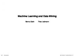
Figure 1. The data mining process.

4


The data mining process and some of its main elements and processes are depicted in Figure 1. In the diagram, processes are portrayed as ovals and rounded boxes. The left side of the diagram illustrates the data access and data preprocessing or representation part of the overall process. This phase transforms the original data (from one or more sources) into an intermediate format. This process may be straightforward or arbitrarily complex, especially when complex background knowledge needs to be incorporated. Currently, it is being discussed if this process can be systematized by means of data warehousing methodology and technology [Dubitzky et al., 2001]. A major obstacle towards this goal is the complexity (logical/structural and temporal) and the global proliferation of the formal background knowledge in biology and life science. The right part in Figure 1 shows the so-called knowledge discovery process. In this process, the pre-processed data is analyzed using a suitable pattern analysis methods. Which method is most suited for the problem at hand depends on the underlying domain, the question being asked, the structure of the available data, and the data mining task that is to be performed. Typical data mining tasks include discriminant analysis, estimation/regression, clustering, association analysis [Hipp et al., 2000], and deviation detection [Arning et al., 1996]. Two of the most common data mining tasks, namely discriminant analysis and clustering, are briefly discussed below. Most of the discussion below is presented from the perspective of discriminant analysis. Both discriminant analysis and cluster analysis are often referred to as classification. However, cluster analysis is quite different from discriminant analysis in that it actually establishes groups (i.e., classes) of objects or entities, whereas discriminant analysis assigns objects to groups that were defined in advance. Clustering seeks a convenient and valid organization (and description) of data and not the generation of rules for separating future data into categories. Thus, cluster analysis is often used when a set of cases or observations is to be divided into "natural" groups. More specifically, clustering is a process or task that is concerned with establishing classes or groups from a set of observations, and with the definition or description of the classes that are identified. Because of this added requirement and complexity, clustering is considered a higher-level process than discriminant analysis. General definitions of both discriminant analysis (also called classification) and clustering (sometimes referred to as automatic classification or partitioning) are provided in Definition 1 and Definition 2 respectively.

Dubitzky et al.

5

Definition 1. Discriminant analysis: Given a universe, U, the subsets (predefined classes) C1, C2, ..., Cn ⊂ U, and the indices 1, 2, ..., i, ..., n ∈ I, then a classifier is a function, f(x): U → I, such that f(x) = i implies x ∈ Ci (that is that x is a member of class Ci). Discriminant analysis is often used to verify or disprove preconceived notions and ideas concerning the relationships in the data (hypothesis testing), or to explain or categorize a certain attribute or property, e.g., tumor type, of the analyzed observations. Definition 2. Cluster analysis: Given a set X with n objects X = {x1, x2, ..., xn} with each object, xi, i = 1 ... n, described by m attributes, xi = (xi1, xi2, ..., xim), determine a classification (grouping, clustering) that is most likely to have generated the observed objects. [Upal & Neufeld, 1996] A frequently applied approach to clustering attempts to produce classes or groups that maximize similarity within classes but minimize similarity between classes. In the context of microarray data analysis, clustering methods may be useful for automatically detecting new subgroups (hypothesis generation) of clinical or biological entities (e.g., tumors, genetic risk groups) in the data [Granzow et al., 2001]. Data mining and data warehousing were first applied on a large scale in so-called customer-oriented businesses including the financial, marketing, retailing, and transportation sector. Typically, in these applications the number of variables is less than 100 and the number of observations ranges from several thousands to several millions. This situation is quite different for microarray data where the number of observations is often very small relative to the number of variables by a factor 10 to 100 or more. Because of this discrepancy it is mandatory to perform cross-validation procedures in order to obtain statistically reliable estimates for the performance of the derived models.

CROSS-VALIDATION In the presence of a large number of observations, cross-validation procedures take up to 90% of the data to construct a discriminant model and estimate the model's future performance by validating it against the remaining observations. The data set for construction of the model is usually called the training set, and that for validation is referred to as the validation set. Given a large number of cases, this procedure yields a statistically sound estimate for gauging the expected performance of the model. However,

6


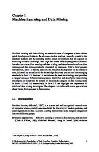
when there is only a limited number of observations, this procedure is not very effective, as (1) the two data sets may be overly biased, and (2) not all available data is used for training. For example, given a two class problem with a total of 100 observations and the absolute class frequencies of F(A) = 80, for class A, and F(B) = 20, for class B, a randomly sampled training set of size 75 may contain no instance of class B at all. Thus, the construction of a good model from this strongly "biased" training set will be difficult. Also, in this example, 25% of the available data is not used for model construction. A way to avoid these problems is n-fold cross-validation. Generally, nfold cross-validation divides the available data set into n folds or subsets. Based on these n data sets, n different models are developed, each using n-1 data sets for training and the remaining data set for validation. The advantage of cross-validation is that it increases the number of data patterns available for training, while using every data pattern available for testing. The diagram in Figure 2 depicts the general approach to cross-validation. In the diagram, the index c = 1, 2, ..., i, ..., n-1, n, refers to the cross-validation fold, and fi(x) denotes the model resulting from the ith cross-validation iteration or fold. For each cross-validation fold, the sets S1 to Sn form a mathematical partition of the original data set.

Figure 2. General model for cross-validation.

Once all n cross-validation iterations have been performed, one can estimate the future performance of the general approach by averaging the performances of the n models on the corresponding validation sets. From

Dubitzky et al.

7

there one may proceed by either selecting the best-performing individual model or by constructing the final model using all the available data. It is important to understand that in the standard cross-validation procedure repeated uniform sampling without replacement is performed. Here, uniform means that each "current" case in the original data set has the same probability of being drawn, and without replacement refers to the fact that once a case is assigned a set (training or validation set) it cannot be assigned or drawn into another set within the same cross-validation fold.

MULTI-MODEL APPROACHES The instability of a prediction method refers to the sensitivity of the final model to small changes in the training set with regard to the prediction accuracy of the model. Small changes in the learning set may lead to large changes in the prediction performance. Typical unstable machine learning methods are decision trees, while, for example, k-nearest neighbor and neural models belong to the class of stable methods. An approach to address the instability problem is to construct multiple models and combine them to make up the final model. There exist three commonly used methods for constructing multi-model systems: boosting, bagging, and stacking [Ng, 1996]. These could be viewed as representatives of a more general framework called data and information fusion [Azuaje et al., 1999]. Boosting, bagging, and stacking deal with creating and combining multiple classifiers but differ in how the classifiers are trained and in how their outputs are combined. Such models often improve accuracy by focusing the learning process on examples in the data that are harder to model than others. We have applied the C5.0 decision algorithm using its boosting option to analyze microarray data in [Dubitzky et al., 2000]. In the following we briefly describe the basic concepts of boosting. Boosting is an algorithm that creates several different models and combines their predictions using a weighted voting scheme (e.g., plurality voting). The elements of a boosting setup and their relationships are depicted in Figure 3. In boosting procedure, N different (perturbed) training set replicas are sampled adaptively (with non-uniform sampling probabilities and with replacement) from the learning set (black box in Figure 3). The predictions of the combined model are generated by means of a weighted voting scheme, where each individual prediction model carries a different weight.

8


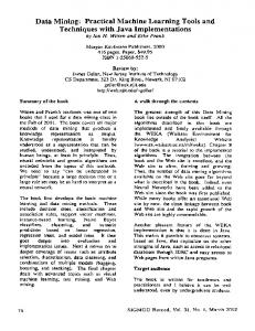
Figure 3. Boosting (thick arrow = uniform sampling, without replacement; double arrow = non-uniform sampling with replacement using sampling probabilities depicted by pi).

The adaptive sampling procedures increase the probability of an instance to be sampled based on the performance of the classifier in the previous iteration. Instances that were most often misclassified are assigned an increased probability for being sampled in the next round. The general algorithm for boosting is governed by the following scheme (which is also illustrated in the diagram in Figure 3): Step 1: Use current (index i) sampling probabilities, pi, and sample with replacement k instances from the learning set (black box labeled Test in the diagram). Step 2: Build current classifier, f'i (x), based on the current training set. Step 3: Establish current classifier's performance by testing it against the learning set (black box) and keep a record of correctly/incorrectly classified cases, and Step 4: Update the sampling probabilities (feedback arrow in upper part of diagram) for each instance based on the classifier's performance and calculate a weight for the classifier also based on its performance (illustrated by the small box in the lower part of the diagram). Step 5: Stop if number of classifiers is reached, otherwise go to Step 1.

Dubitzky et al.

9

In a microarray analysis comprising a total of 72 samples (learning set 27 ALL, 11 AML; and test set of 20 ALL 14 AML) and the expression levels of 7,070 genes, we showed that the C5.0 decision tree algorithm with boosting (10-fold and 20-fold boosting) was superior to the non-boosting version [Dubitzky et al., 2000]. Over a 6-fold cross-validation procedure the non-boosting experiment achieved an average classification accuracy of 84.09%, with 10-fold boosting 91.87%, and with 20-fold boosting 92.98%.

Decision Trees

Figure 4. Example of simple decision tree after learning.

So-called non-parametric models rely heavily on the empirical analysis of large data sets rather than on prior domain knowledge, i.e., domainspecific knowledge about the input-output relationship of the underlying system or problem. The fundamental assumption of non-parametric models is that the consistently observed relationships or patterns in large data sets will recur in future observations. This assumption is crucial as the model attempts to form or learn generalizations based on the presented data. The advantage of non-parametric models is that (1) they do not require a thorough understanding of the underlying system or problem, and (2) they can be used to build arbitrarily complex models, that are highly non-linear and not restricted by human comprehension. Typical non-parametric approaches include decision trees, neural networks, genetic algorithms, and nearest neighbor methods.

10


A decision tree is an approach for generating models that are both descriptive and predictive. The term decision tree is derived from the presentation of the resulting model as a tree-structure (Figure 4 illustrates a very simple decision tree). The example illustrated in Figure 4 shows data (six observations in total: 3 high credit risk, and 3 low credit risk) from a credit risk study involving factors like marital status (Married) and annual earnings (Income), and a decision variable (CreditRisk). The root node at the top of the tree represents all observations. Each intermediate and leaf node contains information about the number of cases at that node and the distribution of the independent variable. Leaf nodes give the classification that applies to all instances that reach the leaf (leaf nodes may not be “pure”). Nodes in a decision tree involve a decision or test about the attributes or variables that reach the node. Typically, this decision is a statistical test on how well an attribute alone classifies the training samples. During training the best attribute is selected and used at this node to evaluate future samples. Also, a descendant of the node is created for each possible value of the selected attribute (in case of discrete variables), unless the node is a leaf node. Continuous variables are first categorized into ranges before branching off a subnode. For example, at the root node in Figure 4 the attribute Income was found to be the best, and the statistical test determined that a split at 30,000 partitioned the underlying cases most effectively. Before we turn to a typical statistical test used to select attributes and generate splits (i.e., create subnodes), we briefly outline the general algorithm used for constructing decision trees. Decision tree learning follows a kind of top-down, divide-and-conquer strategy. The basic algorithm for decision tree learning can be described as follows: 1. Select (based on some measure of "purity" such as entropy, information gain, or diversity) an attribute to place at the root of the tree and branch for each possible value of the tree. This splits up the underlying case set into subsets, one for every value of the considered attribute. 2. Recursively repeat this process for each branch, using only those cases that actually reach that branch. If at any time all instances at a node have the same classification, stop developing that part of the tree. Typical statistical measures used in decision tree algorithms to select an attribute include information gain measures (as implemented in the C5.0 algorithm), and diversity measures (as implemented in the CART algorithm)

Dubitzky et al.

11

[Mitchell, 1997; Breiman et al., 1984]. Here, we illustrate the information gain measure. To define information gain, we first begin by defining another measure, called entropy, that characterizes the (im)purity of a collection of observations. Definition 3. Given a set of predefined classes, C = {c1, c2, ..., cn}, and the indices 1, 2, ..., i, ..., n ∈ I, and the (training) set X with m observations, X = {x1, x2, ..., xm}, with each object, xj ∈ X, described by k attributes and one class cj ∈ C, such that xj = (x1j, x2j, ..., xkj, cj). Then the entropy, entropy(X), of the set X relative to this n-wise classification is defined as n

entropy ( X ) = ∑ − pi log 2 pi

[1]

i =0

where pi is the proportion of X belonging to class ci ∈ C. The measure called information gain, gain(X,A), is simply the expected reduction in entropy caused by partitioning the set of observations, X, based on an attribute A (see equation [2]). gain( X , A) = entropy ( X ) −

∑

Xv

v∈values( A) X

entropy ( X v )

[2]

where values(A) is the set of all possible (discrete) values of attribute A, and Xv is the subset of X for which attribute A has the attribute value v, i.e., Xv = {x ∈ X | A(x) = v}. The strengths of decision trees are: 1. the ability to generate understandable knowledge structures, i.e., hierarchical trees or sets of rules; 2. a low computational cost when the model is being applied to predict or classify new cases; 3. the ability to handle symbolic and numeric input variables; and 4. provision of a clear indication of which attributes are most important for prediction or classification.

The weaknesses of decision trees include: 1. a limited ability to handle estimation or regression tasks where the goal is to predict the value of a continuous variable; 2. error-prone when the number of training examples per class is small; 3. a moderate to high computational cost for growing a decision tree; 4. decision trees generate rectangular classification boxes that may not correspond well with the actual distribution of the underlying regions in the decision space; and 5. without further transformation of the input data, decision trees are not very suitable for learning tasks involving sequential data such as time series. Nowadays there is a plethora of decision tree algorithms available. Two of the most popular and widely used decision tree algorithms are the C5.0 (or its precursor C4.5) [Quinlan & Quinlan, 1997] and CART [Breiman et al., 1984]. Being very similar in many respects, the main differences of these two decision tree algorithms are: 1. The criteria they use to select the candidate attribute for splitting. As mentioned before, C5.0 uses a measure of information gain and CART uses a measure of diversity. 2. The way they split the tree at each node. This is perhaps the most important difference. C5.0 produces trees with varying numbers of branches per node, whereas the CART algorithm performs a binary split at each node and therefore always constructs a binary tree. 3. The pruning method for reducing the complexity of the constructed tree. Generally, CART makes reference to unseen data in order to prune the tree, whereas C5.0 does not consult data beyond the training set. To decide which of the two decision trees to use depends on the underlying task and data. Clearly, an insistence on binary splits (as it is the case with CART), on a variable that is inherently more various, leads to unnecessary complexity in the generated tree. High branching factors (generated by C5.0), on the other hand, lead to a quick reduction of the population of training observations available at each node at lower levels in the tree. This makes further splits less reliable.

12

Dubitzky et al.

13

Neural Networks Artificial neural networks are an emerging computational technology which can significantly enhance a number of applications ranging from robust pattern detection over signal filtering and compression to adaptive control and optimisation tasks. The key properties of neural networks can be summarized as follows: § § § §

adaptive learning: An ability to learn how to do tasks based on the data given for training; self-organization: During learning a neural network can create its own organization or representation of the information it receives; fault tolerance: Noisy data or a partial destruction of the network leads to the corresponding degradation, however, some of the network’s capabilities may be retrained even with major damage; and real-time operation: Neural network computations may be carried out in parallel, and special hardware is being developed which take advantage of this capability. The major strengths of neural networks include: 1. ability to handle a range of problem tasks including classification (discrete outputs) and estimation or regression tasks (continuous outputs); 2. ability to handle many interacting variables (e.g., images) and nonlinear (input-output) behavior of the underlying phenomena; 3. ability to handle symbolic and numeric input variables; 4. provision of an indication (through sensitivity analysis) of which attributes are most important for prediction or classification; and 5. low to moderate computational cost when the model is being applied to predict or classify new cases. The weaknesses of neural networks are: 1. the learned models are described by patterns of connectivity strengths, therefore the rules learned by neural networks cannot be made explicit in symbolic form (the net is the rule); in applications where mere prediction/classification performance is not the only criterion this may be a severe problem; 2. the need to preprocess the inputs in the range of [-1,1] or [0,1] (this is automatically done by most tools);

14

Methods of Microarray Data Analysis 3. the risk of premature convergence to an inferior solution (this is normally addressed by performing a sensible cross-validation procedure); 4. depending on the chosen topology and the learning algorithm, there may be moderate to high computational costs involved in the learning process; and 5. difficulty of defining/finding the optimal network topology for a given task.

Artificial neural networks consist of basic units, called processing elements or neurons, that are modeled on biological neurons. Each processing element has many inputs that it combines into a single output. The learning capability of a neural network is defined by the processing function (called activation function) of the processing elements and the way these elements are connected together, i.e., the network’s architecture or topology. Once a network has been trained, the learned knowledge is represented (stored) in the network by the weights connecting the processing elements.

Figure 5. Neural network elements: (a) topological structure, (b) neurone and activation.

Figure 5 illustrates a simple neural network and its elements. Usually, a network of this type has m output processing elements, PE1, …, PEm, each of which receives n + 1 inputs, namely, in0, in1, in2, …, inj, …, inn from the corresponding input processing elements; in0 is a special input called bias input, it is always set to 1 (for the net in Figure 5-a: m = 2, n = 3). The bias

Dubitzky et al.

15

input, in0, together with the corresponding weights w0i, …, w0m represent thresholds used to control the behavior of the processing elements PE1, …, PEm. The vector C = (in1, in2, …, inj, …, inn) represents an actual case that is to be processed. Each input of a processing element is associated with a set of weights. For example, processing element PE1 is associated with the weights w01, w11, …, wj1 …, wn1. The activation function of each processing element or neurone consists of a combination function and a transfer function (see Figure 5-b). The combination function merges all inputs, and their weights, into a single value. The most common combination function is the weighted sum which is given by equation [3] below. The second part of the activation function is the transfer function. It transfers the output value of the combination function to the output of the processing element. Commonly used transfer functions are the linear, hyperbolic tangent, and sigmoid function; the sigmoid function is defined by equation [4]. xi ( I, W ) =

outi [ xi (I, W )] =

n

∑ w ji in j j =0

1 1 + exp[ − xi (I, W )]

[3]

[4]

In equation [4] (transfer function) the term outi[x(I,W)] denotes the output of the processing element PEi. The transfer function of the processing element PEi determines the element’s output, outi[x(I,W)], based on its input values I = (in0, in1, in2, …, inj, …, inn) and the corresponding weights, W = (w0i, w1i, w2i, …, wji, …, wni), via the combination function xi(I,W) (see equation [3]). The indices 1, 2, …, j, …, n indicate the processing elements or inputs that are connected to PEi. The special bias input, in0, is always fixed to +1, and together with the weight w0i it is used to represent a threshold. Learning in a neural network is the process of setting (adapting) the best weights on the inputs of each processing element. The goal is to produce weights where the output of the network is as close to the desired output as possible for as many examples in the training set as possible. The most common algorithm for doing this is the (error) backpropagation algorithm [Dayhoff, 1996]. The standard implementation of this algorithm proceeds as follows: 1. The network is presented with a training sample or case, defined by the pair (C,class label), and, based on the existing weights, calculates and predicts the outputs (e.g., classification) for the case in question.

16

Methods of Microarray Data Analysis 2. The backpropagation algorithm then determines the error by taking the difference between the calculated outputs and the expected outputs (as provided by a teacher). 3. The error is then fed back through the network and the weights are adjusted (according to some scheme) to minimize the error. 4. Learning normally proceeds until a certain termination criterion is reached. A typical criterion is the prediction accuracy threshold, which is often specified somewhere between 80% and 90%. If too low a value is chosen, the network may not be able to generalize well, so the expected performance on unseen test data will be low. Too high a value entices the net into memorizing or overfitting the training data. As a consequence the net will not perform well on unseen test data since it has failed to generalize from the training data.

Despite the high number of variables (ca. 7,000 genes) and the low number of observations (n=72), we demonstrated that the standard backpropagation algorithm is a useful tool for analyzing microarray data [Dubitzky et al., 2000]. We carried out three experiments with learning accuracy thresholds of 80%, 85%, and 90% respectively over a 6-fold crossvalidation process. The average classification performances were as follows: 93.94%, 94.63%, and 89.70% respectively. Clearly, the decreased performance with the learning threshold of 90% is due to the well-known overfitting effect.

SUMMARY AND CONCLUSION We presented an overview of two widely used machine learning algorithms and two complementary techniques (cross-validation and multimodel approaches) that have been demonstrated to be useful for microarray analysis. The major advantage of these techniques is that they can be readily applied to explore microarray data. In a recent study [Dubitzky et al., 2000] we showed that decision trees (C5.0 implementation with 20-fold boosting) outperformed neural networks (standard backpropagation algorithm). The added advantage of decision trees is that their results can be directly inspected by humans. This may potentially lead to a deeper understanding of the mechanisms governing the underlying biological entities and process. With standard neural networks this option is not readily available. Perhaps one of the most important drawbacks of the presented methods is that they do not readily lend themselves to single-event probabilities or statistical

Dubitzky et al.

17

confidence intervals in connection with their predictions. Clearly, much more analysis, experiments, and statistical and biological validation is necessary to establish a comprehensive set of properties on data mining and machine learning approaches to microarray analysis.

References Arning, A., Agrawal, R., Raghavan, P., "A linear method for deviation detection in large databases", Proc. 2nd Int'l Conference on Knowledge Discovery and Data Mining, pp164-169, 1996. Berry, M.J.A. and Linoff, G., "Data Mining Techniques: For Marketing, Sales, and Customer Support", John Wiley & Sons, 1997. Breiman, L., Friedman, J.H., Olshen, R.A., Stone, C.J., "Classification and Regression Trees", Wadsworth, Monterey, CA, 1984. Chen J.J., Wu R., Yang P.C., Huang J.Y., Sher Y.P., Han M.H., Kao W.C., Lee P.J., Chiu T.F., Chang F., Chu Y.W., Wu C.W., Peck K., "Profiling expression patterns and isolating differentially expressed genes by cDNA microarray system with colorimetry detection", Genomics, 1;51(3), pp313-24, 1998. Dayhoff, J.E., “Neural Network Architectures: An Introduction”, Thomson Computer Press, 1996. Dubitzky, W., Granzow, M., Berrar, D., Bulashevska, S., Conrad, C., Gerlich, D., Eils, R., "A Comparison of Symbolic and Subsymbolic Machine Learning Approaches to Molecular Classification of Cancer and Gene Identification", in Critical Assessment of Techniques for Microarray Data Mining (CAMDA-2000), pp12-13, 2000. (extended abstract) Dubitzky, W., Krebs, O., Eils, R., "Minding, OLAPing, and Mining Biological Data: Towards a Data Warehousing Concept in Biology", Proc. Network Tools and Applications in Biology (NETTAB), CORBA and XML: Towards a Bioinformatics Integrated Network Environment, pp78-82, Genoa, Italy, 2001. Golub T.R., Slonim D.K., Tamayo P., Huard C., Gaasenbeek M., Mesirov J.P., Coller H., Loh M.L., Downing J.R., Caligiuri M.A., Bloomfield C.D., Lander E.S., "Molecular classification of cancer: class discovery and class prediction by gene expression monitoring", Science 286(5439) pp531-537, 1999. Granzow M., Berrar D., Dubitzky W., Schuster A., Azuaje F. and Eils R., "Tumor Classification by Gene Expression Profiling: Comparison and Validation of Five Clustering Methods ", in ACM-SIGBIO Letters, 2001. (in press) Hipp J., Güntzer U., Nakhaeizadeh G., Algorithms for Association Rule Mining: A General Survey and Comparison, SIGKDD Explorations, 2(1), pp58-64, 2000. Mitchell, T.M., "Machine Learning", McGraw-Hill, Singapore, 1997. Newton M.A., Kendziorski C.M., Richmond C.S., Blattner F.R., Tsui K.W., "On differential variability of expression ratios: improving statistical inference about gene expression changes from microarray data", J Comput Biol., 8(1), pp37-52, 2001 Ng, K., "An experimental comparison of stacking, bagging, boosting for combining ensembles of radial basis function classifiers", Term Project 9.520, Spoken Language Systems Group, Laboratory for Computer Science, Massachusetts Institute of Technology, 1996. Quinlan, J.R. and Quinlan, R., "C4.5: Programs for Machine Learning", Morgan Kaufmann Series in Machine Learning, 1997. Upal, M.A. and Neufeld, E., "Comparison of unsupervised classifiers", in Proc. of the First

18


International Conference on Information, Statistics and Induction in Science, pp342-353, World Scientific, Singapore, 1996. Voit E.O. & Radivoyevitch T., "Biochemical systems analysis of genome-wide expression data", Bioinformatics, 16(11), pp1023-37, 2000. Witten, I.H. and Frank, E., "Data Mining: Practical Machine Learning Tools and Techniques with Java Implementations", Morgan Kaufmann Pub., 2000.