1 Associative Data Storage and Retrieval in Neural ... - Semantic Scholar

1 Associative Data Storage and Retrieval in Neural Networks Gunther Palm 1 Friedrich T. Sommer 2

ABSTRACT Associative storage and retrieval of binary random patterns in various neural net models with one-step threshold-detection retrieval and local learning rules are the subject of this paper. For dierent heteroassociation and auto-association memory tasks, specied by the properties of the pattern sets to be stored and upper bounds on the retrieval errors, we compare the performance of various models of nite as well as asymptotically innite size. In innite models, we consider the case of asymptotically sparse patterns, where the mean activity in a pattern vanishes, and study two asymptotic delity requirements: constant error probabilities and vanishing error probabilities. A signal-to-noise ratio analysis is carried out for one retrieval step where the calculations are comparatively straightforward and easy. As performance measures we propose and evaluate information capacities in bits/synapse which also take into account the important property of fault tolerance. For auto-association we compare one-step and xed-point retrieval that is analyzed in the literature by methods of statistical mechanics.

1.1 Introduction and Overview With growing experimental insight in the anatomy of the nervous system as well as the rst electrophysiological recordings of nerve cells in the rst half of this century, a new theoretical eld was opened, namely, the modelling of the experimental ndings at one or a few nerve cells, leading to very detailed models of biological neurons 1]. But dierent from most biological phenomena, where the macroscopic function can be understood by revealing the cellular mechanism, the function of the nervous system as a whole turned out to be constituted by the collective behaviour of a very large number of nerve cells and the activity of a large fraction of cells, a 1 Abteilung Neuroinformatik, Fakultat fur Informatik, Universitat Ulm, Oberer Eselsberg, D-89081 Ulm, Germany 2 C. und O. Vogt Institut fur Hirnforschung, Universitat Dusseldorf, Moorenstr. 5, D-40225 Dusseldorf, Germany

ii

1. Associative Data Storage and Retrieval in Neural Networks

whole activity pattern, had to be considered instead. The modelling had to drop the biological faithfullness at two points: on the cellular level the models had to be simplied such that a large number of nerve cells could be described and on the macroscopic level the function had to be reduced to simple activity pattern processing like pattern completion, pattern recognition or pattern classication allowing a theoretical description and quantication. McCulloch and Pitts 2] argued that due to the \all or none" character of nervous activity the neurophysiological ndings can be reproduced in models with simple two-state neurons, in particular, in associative memory models which exhibit binary activity patterns. In the ftees and sixtees small feed-forward neural nets have been suggested for simple control tasks, among them the associative memory 3], 4], or the simple perceptron 5]. All these models employ one-step retrieval which means that in one parallel update step the initial or input pattern is transformed to the output pattern. Such models which contain no feed-back loops will be the main subject of this paper. Little, who introduced the Ising-spin analogy of the neural states 3 6], opened the door to analyzing the feed-back retrieval process in neural nets with methods of statistical mechanics. The analysis which was develloped during the seventies 7] for lattices of coupled spins with randomly distributed interactions to describe spin glasses could be applied successfully to
xed-point retrieval in an associative memory 8]4 . In xed-point retrieval, the retrieval process is iterated until a stable state is reached. This method has been described in several recent books, e. g. van Hemmen and Kuhn 9], Amit 10] and Hertz, Krogh, and Palmer 11]. This paper takes as starting point a larger class of simple processing tasks: the association between members of binary pattern sets. Depending on properties of the randomly generated pattern sets we will characterize dierent memory tasks (Sect. 1) and concentrate on the question how a neural model has to be designed to yield optimal performance. We consider feed-forward neural associative memory models with onestep retrieval (Sect. 2). To keep our model as variable as possible, Ising-spin symmetry of the neural states is not assumed and arbitrary local learning rules are admitted to form the synaptic connections. One-step retrieval can be analyzed by elementary probability theory and it is compatible 3 The two states of a binary neuron are identied with up and down states of a spin particle in the Ising model, the synaptic couplings correspond to the spin-spin interactions. 4 Pattern completion with xed-point retrieval in a neural net can be treated like relaxation in a solid, once the storage process has determined the dynamics. The macroscopic observables of the system (corresponding to specic heat, conductivity or magnetization in solids) are then the overlaps to stored patterns, or equivalently the recall errors.

Gunther Palm , Friedrich T. Sommer

iii

with a larger class of memory tasks, not only pattern completion. On the other hand, as we will discuss, in cases of pattern completion a feed-back retrieval model is preferable. Section 3 contains the detailed signal-to-noise ratio analysis where we have included most of the calculations because the intention of this work is to provide not only results but also the methods. Another important question concerns the judgement of the performance of dierent memory models. Unfortunately, in the literature a lot of dierent measures are used. Instead of staying with the mean retrieval errors obtained from the analysis, we apply elementary information theory to the memory process, leading us to the denition of information capacities which allow to compare models with dierent memory tasks (Sect. 4). In Sect. 5 we evaluate these performance measures for the various models. The last section resumes the previous sections and points out the relations to the literature. It compares one-step and xed-point retrieval, taking advantage of the works based on methods of statistical mechanics. The results of the dierent approaches, which seem to be quite incoherent at rst sight, turn out to be not only comparable but also consistent.

1.1.1 Memory and Representation A memory process can often be considered as a mapping from one set of events into another set of events as a trivial example one may think of the problem how to establish a phone line to a friend. To solve the problem one has to map the friends name to his phone number. For the construction of a memory device like a phonebook which helps you with this problem one rst has to map or to code the events \the friend's name" and the \his phonenumber" into symbols, in this case strings of letters and numbers, which can be written and read by a user. This mapping will be called the representation of the events. The memory device has to store these pairs of strings in some way. It can solve the problem if the representation maps the events into unique data strings. Thus a given set of patterns specify the memory task which a memory device has to solve. Without loss of generality we focus on binary patterns as data strings. A binary pattern is a string containing only two types of elements, for instance \B" and \W" (for black and white pixels). We will restrict ourselves to such pattern sets where every member has approximately the same ratio p beween the number of \B" and \W" digits. We call a pattern distributed, if both fractions of pixels have more than one member. Throughout this work we distinguish three dierent patterns types: A singular pattern has only one \B" digit out of m ; 1 \W" digits, if m is the number of digits in the pattern. A singular pattern is by denition not distributed. A sparse pattern is distributed but the ratio p between the number of \B" and \W" digits satises p 0] ' G ;#r] (1.15) p Rx with the normal or Gaussian distribution G x] := (1= 2 ) e x2 =2 dx. To obtain explicit values for the error probabilities we now have to analyze the signal and noise term in (1.13) for the dierent ensembles of input patterns and dierent learning rules (Section 2.2). For input ensembles we are interested in the mean retrieval errors where for every input the threshold has been set in the optimal way according to the number of active input digits n1 . We insert the signal-to-noise ratio averaged over an input ensemble into (1.14) and consider a xed threshold setting which is equal for all input patterns. As to binary storage we take this result as an approximation for the individual threshold adjustment which is equivalent to an exchange of the expectations of the pattern average and the input average in the calculation. ;

;1

Signal-To-Noise Calculation Again we discern the three cases of addressing described in Sect. 1.3.1. a) For the faultless address xk as input the signal is sharply determined as s1 ; sa = n1 (r4 ; r3) ; (m ; n1)a(r2 ; r1 ): The noise decouples into a sum of (M ; 1) independent contributions corresponding to the storage of the pattern pairs (xl  yl ) with l 6= k. For every pair the input xk generates a sum of n1 random variables R(x y) and of (m ; n1) random variables aR(x y) at a neuron j. The variable R(x y) = R(xli yjl ) is the four-valued discrete random variable (1.4) with the distribution: (1 ; p)(1 ; q) p(1 ; q) (1 ; p)q pq. With E(R) and 2 (R) denoting expectation and variance of R(x y) a simple (but for 2 (N) tedious) calculation yields E(N) = (M ; 1) n (1.16) 1 + (m ; n1 )a] E(R)   2 (N) = (M ; 1) Q1 2 (R) + Q2 CovRiRh ] (1.17)

Gunther Palm , Friedrich T. Sommer

xv

where we have used the abrevations Q1 := n1 + (m ; n1 )a2 Q2 := n1(n1 ; 1) + 2an1 (m ; n1 ) + a2 (m ; n1 )(m ; n1 ; 1) CovRiRh ] = q(1 ; q) p(r4 ; r3 ) + (1 ; p)(r2 ; r1 )]2
The covariance term: CovRiRh ] := Cov R(xli  yjl )R(xlh  yjl ) measures the dependency between two contributions in the i-th and h-th place of the column j upon the synaptic matrix. b) If we average over the ensemble of perfect input patterns we can use again for large m the approximations n1 =m ' (n1 ; 1)=m ' (n1 +1)=m ' p and (M ; 1)=m ' M=m and obtain E(s1 ; sa ) = m p(r4 ; r3) ; (1 ; p)a(r2 ; r1)] E(N) = (M ; 1)mE(R) In equation (1.17) we have to insert

(1.18)




Q1 = m p + (1 ; p)a2  Q2 = m2 2 : (1.19) c) Finally, we consider the ensemble of noisy address patterns. In this case E(s1 ; sa ) = m p(p + (1 ; p )a)(r4 ; r3) ; (1 ; p)a(r2 ; r1)] : (1.20) In the description of the noise we only have to replace in (1.18) and (1.19) p by pp and  by  . 0

0

0

0

0

0

Signal-to-noise Ratios for Explicit Learning Rules Regarding (1.17) and (1.18) we observe that the signal-to-noise ratio is the same for the rules R and bR + c, where c is an arbitrary and b is a positive number. Two rules that dier only in this way, will be called essentially identical. Thus we may denote any rule R as R = (0 r2 r3 r4): (1.21) The following formulae are written more concisely if we introduce instead of r2 r3 r4 the mutually dependent parameters

:= r4 ; r3 ; r2   := r2 + p  := r3 + q: In this notation the variance of the rule becomes 2 (R) : = E(R2 ) ; (E(R))2 = 2 p(1 ; p) + 2 q(1 ; q) + 2 p(1 ; p)q(1 ; q)

xvi

1. Associative Data Storage and Retrieval in Neural Networks

In the description of the input ensemble we transform from the parameters p a to the quantities p , see (1.7). The signal-to-noise ratio averaged over perfect address patterns b) is then obtained from equation (1.13) as  + (1 ; )p ]2 r2 = (m=M) p + ( ; p)2=(1 : ; p)]2 (R) + mq(1 ; q)2 2

(1.22)

Averaged over noisy address patterns c) we obtain equivalently (1 ; )pp ]2 r 2 = (m=M) pp + ( ; pp )2=(1 ;+pp )] 2 (R) + mq(1 ; q) 2 2 (1.23) with the denition for  taken from (1.8). 0

0

0

0

0

0

0

0

0

Optimal Learning Rule The expression (1.22) invites to optimize the signal-to-noise ratio in terms of the three parameters ,  and so as to yield the optimal learning rule R0. The parameter appears only in 2 (R) in the denominator. We rst minimize 2 (R) with = 0 and obtain  + (1 ; )p ]2 m) r2 = ( M q(1 ; q) fp + ( ; p)2 =(1 ; p)]2 + 2 p(1 ; p)] + m2 2 g :(1.24) The (large) factor m in the second term of the denominator in eq. (1.24) makes this term dominating unless at least one of the other factors  or  vanishes. At a rst sight we have to distinct two cases which dier with respect to the average activity  of the input patterns: Either  stays away from zero, then it is optimal to choose  = 0 (case 1). Or  ! 0 fast enough to make the second term negligible in the sum of the denominator in eq. (1.24). However, if we insert  = 0 in (1.24), again  = 0 turns out to be the optimal choice (case 2). Thus both cases leave us with  = 0 and = 0 and yield the covariance rule as general optimal rule R0 = (pq ;p(1 ; q) ;q(1 ; p) (1 ; p)(1 ; q)):

(1.25)

The condition  = 0 will occur several times in the sequel, and will be referred to as the condition of zero average input activity. In particular, for p = 0:5 it implies a = ;1 and for p ! 0 this implies a ! 0. This condition,

Gunther Palm , Friedrich T. Sommer

xvii

which is equivalent to a = ;p=(1 ; p) or to p = ;a=(1 ; a) xes the optimal combination between input activity and the model parameter a. For arbitrary p and a in the input patterns and for arbitrary , the optimal signal-to-noise ratio is evaluated by inserting R0 in eq. (1.24), 2p : (1.26) r02 = (m=M) q(1 ; q) p + ((1;;p))2 =(1 ; p)] (1 ; p) Transforming back from  to a we obtain ; p)(1 ; a)2 r02 = (m=M) p +p(1 (1.27) (1 ; p)a2 ] q(1 ; q) : Insertion of the zero average input condition  = 0 in (1.26) yields the optimal signal-to-noise ratio (1.28) r02 ' Mq(1m; q) :

Optimizing the signal-to-noise ratio for noisy addresses c), eq. (1.23) leads to the same optimal rule (1.25). Then the signal-to-noise ratio value for perfect addressing is reduced from the noise in the input patterns. For the optimal rule R0 with  = 0 it is given by p)p 2 r2: r02 ' p (1;;2pp (1.29) +p 0 For learning rules with  6= 0 which have a nonzero covariance term only  = 0 can supress the m2 term in the variance of the noise. Therefore,  6= 0 and  6= 0 lead to vanishing r as m ! 1. A little algebra shows that learning rules with  6= 0 and nite also yield a vanishing r. In conclusion all suboptimal rules need  = 0 to achieve a nonvanishing r. 0

0

0

0

Hebb and Agreement Rule If we compare the Hebb rule and the agreement rule to the optimal learning rule R0 we realize, that in general both rules are suboptimal. But nevertheless, for p = q = 0:5 the optimal rule becomes equal to the agreement rule: R0 = (0:25 ;0:25 ;0:250:25) and for p q ! 0 the Hebb rule is approximated by the optimal rule: R0 ! H. By equation (1.22) one can compute the signal-to-noise ratio for these rules, the results for  = 0 you nd in Table 1. As expected, the Hebb rule becomes essentially identical to R0 for p q ! 0. In the a = 0 model, where the parameter a is not adjusted to guarantee  = 0 we need a stricter sparseness in the address patterns: mp2 ! 0 to provide  ! 0 fast enough to preserve the essential identity between H and R0. By comparing the r2 values corresponding to the dierent rules in Table 1 we will derive the performance analysis of Hebb and agreement rule (see Section 5.2 and 5.4) from the analysis of R0 carried out in this section.

xviii

1. Associative Data Storage and Retrieval in Neural Networks TABLE 1.1. Squared signal-to-noise ratios r2 (m M p q) for  = 0.

Optimal rule R0 Hebb rule H

r2 =

m Mq(1 ; q)

m(1 ; p) Mq(1 ; pq)

Agreement rule C

8mp(1 ; p) M p(1 ; q) + (1 ; p)q]

Summary With incremental storage procedure the signal-to-noise ratio analysis of one-step threshold-detection retrieval led to the following results: If a rule R yields the signal-to-noise ratio r then any rule bR+c, with b positive yields the same signal-to-noise ratio. We call these rules essentially identical. For any rule R the best combination of the parameters p and a is given by the zero average input condition  = p + (1 ; p)a = 0. The maximal signal-to-noise ratio r0 is always achieved for the covariance rule R0 (1.25). For increasing  the value r0 continously decreases and reaches r0 = 0 at  = 1. Every rule essentially dierent from R0 has zero asymptotic signalto-noise ratio, if the condition  = 0 is violated. The Hebb rule becomes essentially identical to R0 for memory tasks with q ! 0 and p ! 0, i.e., for sparse address and content patterns. The agreement rule is equal to R0 for p = q = 0:5. Storage of extensively many patterns, i.e., M=m > 0 as m ! 1: In this case R0 and H achieve asymptotically vanishing errors (r ! 1) for memory tasks with sparse content patterns: q ! 0 as m ! 1. The agreement rule A only achieves r = const as m ! 1.

1.4 Information Theory of the Memory Process How can the performance of an associative memory model be measured ? In our notation a given memory task species the parameters: p q M p  ea  e1. From the signal-to-noise ratio analysis we can determine for randomly generated patterns the maximal number of pattern pairs M , for which the required error bounds ea  e1 are still satised. Then the rst idea is to compare the M to the number of neurons used in the memory model. This quotient of patterns per neuron = M =n is used in a lot of works 0







Gunther Palm , Friedrich T. Sommer

xix

but this measure disregards the parameter q used in the random generation of the content patterns as well as the whole process of addressing. In the following we use the description of elementary information theory to nd performance measures for the memory task and compare them with the size of the storage medium, viz., the number of synaptic connections n m.

1.4.1 Mean Information Content of Data Every combination of a memory problem and a coding algorithm will lead to a set of content patterns which exhibit in general very complicated statistical correlations. For a set of randomly generated patterns S which we have used to carry out the signal-to-noise ratio analysis each digit was chosen independently. The mean information contained in one digit of a pattern is then simply given by the Shannon information 40] for the two alternatives with the probabilities p and 1 ; p i(p) := ;p log2 p ; (1 ; p) log2 (1 ; p) and the mean information content in the set of randomly generated content patterns S C is I(S C ) = Mn i(q) where q is the ratio between 1- and acomponents in each content pattern. The pattern capacity compares the mean information content of the content patterns with the actual size m n of the storage medium and is dened as P(m n) := max fI(S C )g=nm = M i(q)=m: (1.30) M 

Here M equals the maximum number of stored patterns under a given retrieval quality criterion. The denition (1.30) is an adequate measure of how much information can be put in the memory but not at all of how much can be extracted during the retrieval. A performance measure should also consider the information loss due to the retrieval errors. 

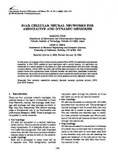
1.4.2 Association Capacity The memory can be regarded as noisy information channel consisting of two components (see Fig. 2): The channel input is the set of content patterns S C and the channel output is the set of recalled content patterns S~C a%icted with the retrieval errors. The two components correspond to the storage process where the sets S A and S C are transformed into the synaptic matrix and to the retrieval process where the matrix is transformed into a set of memory output patterns S~C . The retrieval error probabilities specify the deviation of S~C from S C and thus the channel capacity.

xx

1. Associative Data Storage and Retrieval in Neural Networks

T (S~C S C )

............................................................................................................................................................................ ................................ .................. .................. .............. ............. ........... . . . . . . . . . . . .......... ... . . . . . . . ....... . . . . . . ...... . ..... .......... ........ ........ ................. .............. .......................................... . . . . . . . . . . . . . . . . . . . . . . . . . . . . . . . . . . . . . . . . . . . . . . . . . . . . . . . . . . . . . . . . . . . . . . . . . . . . . . . . . . . . . . . . . . . . . . . . . . . . . . .... . . . . . . . . .................. ....... ....... ...... ...... .................

(S A, S C )

mem. task

Storage

M

mem. matrix

Retrieval, Adressing

S~C

ret. output

FIGURE 1.2. Output capacity: Information channel of storage and retrieval. (The abbrevations \mem." for memory and \ret." for retrieval have been used.)

The capacity of an information channel is dened as the transinformation that is contained in the output of the channel about the channel's input. The transinformation between S~C and S C can be written T(S~C  S C ) = I(S C ) ; I(S C j S~C ) (1.31) where the conditional information I(S C j S~C ) is subtracted from the information content in S C . It describes the information necessary to restore the set of perfect content patterns S C from the set S~C . For random generation of the data we obtain k k (1.32) I(S C j S~C )=nm = M m I(yi j y~i ) with the contribution of one digit I(yik j y~ik )=Prob~yik = 1]i(Probyik = 0 j y~ik = 1]) +Prob~yik = 0]i(Probyik = 1 j y~ik = 0])  ; q)ea =q(1 ; e1 ) + (1 ; q)ea ] i q(1 ; (1 e1 ) + (1 ; q)ea   1 +qe1 + (1 ; q)(1 ; ea )] i qe + (1 ;qeq)(1 : (1.33) ; ea ) 1 Now we dene the association capacity as the maximal channel capacity per synapse A(m n) := max T(S~C  S C )=mn = P(m n) ; Mm I(yik j y~ik ): (1.34) M The capacity of one component of the channel is an upper bound for the capacity of the whole channel: The capacity of the rst box in Fig. 2 will be called storage capacity (discussed in 41]). The maximal memory capacity that can be achieved for a xed retrieval procedure (i.e. xing only the last box in Fig. 2) will be called the retrieval capacity. 

Gunther Palm , Friedrich T. Sommer

xxi

T (S~C S C )

....... ....... ....... ....... ...... ...... ....... ....... ....... ....... ....... ....... ....... ...... ....... ....... ....... ...... . ...... . . ....... ... ...... . . . . ....... . ... . . . ...... ..... . ..... ..... ........ ........ ........ ........ ................. ....................................... ...................................... ....................................... ....................................... ...................... ... ... .. ...

SC

mem....task

Storage

M

mem. matrix

Retrieval

S~C ret. output ..

. .. . . ....................... .... ...... ....... ..... .. ......... . . . . . ............. ....... ... . . . . . . . . . . . . . . . . . . . . . . . .... ....... . ... ....... ....... ....... ........................... ....... ...... ..... . ...................... ................................................................................. .................

^C

S Addressing T (S~C S C ) ; T (S^C S C )

T (S^C S C )

FIGURE 1.3. Completion capacity: Information balance for autoassociation. (The abbrevations \mem." for memory and \ret." for retrieval have been used.)

1.4.3 Including the Addressing Process The dened association capacity is a quality measure of the retrieved content patterns but the retrieval quality depends on the properties of the input patterns and on the addressing process. Of course, maximal association capacity is obtained for faultless addressing and with growing addressing faults (decreasing probability p ) the association capacity A decreases because the number of patterns has to be reduced to satisfy the same retrieval error bounds. To include judgement of addressing fault tolerance for hetero-association we have to observe the dependency A(p ). For auto-association where S A = S C we will consider the information balance between the information already put into the memories input and the association capacity (see Fig. 3). This dierence gives the amount of information really gained during the retrieval process. We dene the completion capacity for auto-association as the maximal dierence of the transinformation about S C contained in the output patterns and contained in the noisy input patterns S^A , n o C(n) := max T( S C j S~C ) ; T(S C j S^C ) =n2 : (1.35) ^C 0

0

S

From (1.31) we obtain n o C(n) = max I( S C j S^C ) ; I(S C j S~C ) =n2 ^C S






= max M I(yik j y^ik ) ; I(yik j y~ik ) =n: p 

0

(1.36)

In (1.36) we have to insert again the maximum number of stored patterns M and the conditioned information to correct the retrieval errors cf. eq. (1.33). In addition the one-digit contribution of the conditioned information necessary to restore the faultless address patterns S A from the noisy input patterns S^A is required. It is given by   p(1 ;p) k k (1.37) I(yi j y^i ) = (1 ; pp )i 1 ; pp : 

0

0

0

xxii

1. Associative Data Storage and Retrieval in Neural Networks

Note that for randomly generated content patterns, i.e., with complete independence of all the pattern components yik , one usually reaches the optimal transinformation rates and thus the formal capacity.

1.4.4 Asymptotic Memory Capacities In Sect. 3 we have also analyzed the model in the thermodynamic limit, the limit of diverging memory size. For asymptotic values for the capacities in this limit we will not only examine memory tasks where the delity requirement remain constant. We will examine the following asymptotic
delity requirements on the retrieval which distinguish asymptotically different ranges of the behaviour of the quantities ea and e1 with respect to q ! 0 as m n ! 1: The high-delity or hi-
requirement: e1 ! 0 and ea =q ! 0. Note that for q ! 0 the hi- requirement demands for both error types the same behaviour of the ratio between the number of erroneous and correct digits in the output: da ' d1 ! 0 with the error ratios dened by da := ea =q and d1 := e1 =(1 ; q). The low-delity or lo-
requirement: e1 and ea stay constant (but small) for n ! 1 With one of these asymptotic retrieval quality criteria the asymptotic capacities P , A and C are dened as the limits for n m ! 1 and n ! 1, respectively.

1.5 Model Performance 1.5.1 Binary Storage Output capacity In this memory model the probability p0 = Prob(Mij = 0) is decreased, if the number of stored patterns is increased. Since obviously no information could be drawn from a memory matrix with uniform matrix elements we will exclude the cases p0 = 1 and p0 = 0 in the following. For faultless addressing the maximal number M of patterns which can be stored for a given limit on the error probabilities can be calculated by (1.9) and (1.10),
ln 1 ; (ea )1=mp lnp 0] (1.38) M = ln1 ; pq] = ln1 ; pq] : From (1.34) we obtain for e1 = 0 and e := ea ; ( ln1 ; p0]) 1 . Inserting (1.42) in (1.40) we obtain the inequality ln1 ; p0 ] (1.43) M < m lnp;0q] lnq] which can be put into (1.39) yielding for p0 = 0:5 and m ! 1 the maximal association capacity: A ' 0:69 bits/syn. Note that for auto-association and for hetero-association with p = q m = n equation (1.42) implies that p / lnn]=n (1.44) and  2 n M / lnn] : (1.45) The relation (1.45) has already been obtained in 42, 43] for sparse memory patterns with arbitrary learning rules by regarding the space of all possible synaptic interactions cf. Sect. 1.6.3. For singular address patterns and arbitrary q = const, however, errorfree retrieval is possible for M  m, which is the combinatorical restriction for nonoverlapping singular patterns. In this case, with (1.39) an association capacity of A = i(q)  1 bits/synapse is obtained. For constant p equation (1.42) demands asymptotically empty content patterns: q / exp (;mp=u), leading to vanishing association capacity. For singular content patterns the combinatorial restriction M  m also yields vanishing association capacity. ;









Fault Tolerance and Completion Capacity In the case of noisy input patterns (1.12) the hi- condition becomes : ea =q = exp (mpp ln1 ; p0] ; lnq]) ! 0. Like in the preceeding subsection we obtain the maximal number of patterns by M = p M where M is the value for faultless addressing (1.43). Thus for hetero-association the association capacity exhibits a linear decrease with increasing addressing fault: A(p ) = p A. 0

0

0

0

0





Gunther Palm , Friedrich T. Sommer

0.2

0.2




m = 512




m = 512

- - m = 4096 | m = 1048576

- - m = 4096 | m = 1048576

C 0.1 0.0

... ... ... .... ....... . ..... ... ......... ...... . .. ....... ....... ....... ... . .... .. . ... ....... ....... ..... . ....... ... ... . ... .... .... ..... .. ... . .... . . . ..... .. .... . .. .. . ...... .. .... ... .. ...... .... . . . . . . ......... . . ... ... .............................................................................................

0.008 p

.... .. .... ...... .. .............. ..... .. .. ..... .. . ..... ...... ... . ........ .. .. . . .. ... ..... ....... ..... .. ....... . .. .. .... . ...... .... .. ..... . ... .... .. .... ..... .... .. ... .. ..... . ...... .. .. ... .. ....... .... . . . . . ........ . . . .. . ...............................................................................................

C 0.1

d = 0:01

0.000

xxv

0.0

0.016

d = 0:05

0.000

0.008 p

0.016

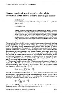
FIGURE 1.6. Binary storage in nite memory sizes: Completion capacity C in bits/syn for two lo- values, the maximum has always been achieved for addressation with p = 0:5. 0

For auto-association with the hi- requirement the retrieval error term in the completion capacity (1.36) can be neglected like in the association capacity and we obtain for p ! 0    p(1 ;p ) C = max (M =n)(1 ; pp )i 1 ; pp p   lnp 0 ] ln1 ; p0 ] p (1 ; p ) = max = 0:17 bits/syn (1.46) p ln2] 0

0

0

0

0

0

0

0

for p0 = 0:5 and p = 0:5. In Fig. 1.6 the completion capacity is plotted against p for three nite memory sizes and for the constant error ratios a): d = ea =p = 0:01 and b): d = 0:05. The optimum is always obtained for p = 0:5. 0

0

1.5.2 Incremental Storage Output capacity For faultless addressing, zero average input and the optimal rule R0, the maximal number of stored patterns for a given signal-to-noise ratio value r is obtained from equation (1.28) M = m=(r2 q(1 ; q)): (1.47) If the threshold setting provides ea =q = e1 =(1 ; q) =: d, the association capacity can be computed for small xed values of the error ratio d from (1.34) and (1.47) 2 qd] + log2 (1 ; q)d]g A ' i(q) + q(1 ; q)d rf2log (1.48) q(1 ; q) 

xxvi

1.2

0.8 0.4 0.0

1. Associative Data Storage and Retrieval in Neural Networks

0.4

... ... ...



... ... ... ... .... 0 ..... .... ...... .... ..... .... ....... . ..... ............ . . .......... ..... ................... ....... ....... . ........................... ............... ...... ............................................................... ...... ...... ... ....... ....... .......

rule A - - rule H | rule R

O 0.2 0.0

0.0 0.1 0.2 0.3 0.4 0.5 p

.... . .......... .. .......... .. . ............. .. ..... ............................... ...................................................... .. ....... .................. ...... .. ....... ............ .. .................. .. . . . . . . . . . ... . ....... .... .... ... ....... . ...... ....... ... .... ... ...... .. ... ....

0.0 0.1 0.2 0.3 0.4 0.5 p

FIGURE 1.7. Model with incremental storage, fulllled condition of zero average input and m n ! 1 : Number of stored patterns  (left) and asymptotic output capacity A in bits/synsapse (right) for p = q with the lo- requirement d = 0:01. The optimal rule R0 is approached by the agreement rule A for p = 0:5 and by the Hebb rule for p ! 0. For p ! 0, the lo- output capacity values of optimal and Hebb rule reach but do not exceed the hi-value of A = 0:72 bits/synapse (This can only be observed, if the p scale is double logarithmic see Fig. 5 in Pa91]).

With substitution of r = G 1 qd] + G 1 (1 ; q)d] in (1.48) we obtain the association capacity for the rule R0 for a constant d error ratio, the lo- requirement. (G 1 x] is the inverse Gaussian distribution.) In Fig. 1.7 we display the association capacity values for optimal, Hebb and agreement rule, the latter two obtained by comparison of the signal-to-noise ratios in Table 1, Sect. 1.3.4. The hi- requirement can only be obtained for r ! 1 as m ! 1 in (1.47) which is possible either for M =m ! 0, leading to vanishing association capacity or for q ! 0, the case of sparse content patterns, which we focus on in the following. We now choose a diverging signal-to-noise ratio by p (1.49) r = ;2 lnq]=#: The threshold has to be set asymmetrically: # ! 1 because for sparse patterns ea =e1 ! 0 is demanded. (This implies q = exp; (#r)2 =2], yielding with Appendix 2: ea =q ' ( r2 =2) 1=2 ! 0. If the threshold # approaches 1 slowly enough that still (1 ; #)r ! 1 holds, then also e1 ! 0 is true and the hi- requirement is fulllled.) With vanishing e=q equation (1.48) simplies asymptotically to 2 e] A  P + 2elog 'P r2 Again the information loss due to retrieval errors can be neclected due to the high delity requirement. ;

;

;



;

Gunther Palm , Friedrich T. Sommer

xxvii

Inserting (1.49) in (1.47) we obtain for zero average input and the optimal rule R0 M = m= (;2q(1 ; q) lnq])

(1.50)



which again can also be found with the Gardner method 42, 43] cf. Sect. 1.6.3. With (1.50) and (1.30) we obtain as asymptotic association capacity with the hi- requirement: A = 0:72 bits/syn. In contrast to the model with binary storage { where only for sparse content and address patterns a positive association capacity has been obtained { with incremental storage an association capacity A = 0:72 bits/syn is achieved even for memory tasks with nonsparse address patterns. However, for f0 1g-neurons we are again restricted to sparse address patterns because for nonsparse address patterns the zero average input condition cannot be satised. With singular address or content patterns which are no interesting cases for associative memory as we will discuss in Sect.1.6.1, incremental and binary storage form the same memory matrix and achieve exactly the same performance see last part of Sect. 1.5.1. Fault tolerance and Completion Capacity For hetero-association with noisy addressing we obtain the association capacity for zero average input and R0 by using equation (1.29) (remember that r2 / m=M) p)p 2 A: A(p ) = p (1;;2pp (1.51) +p 0

0

0

0

For p = 0:5 this implies A(p ) = p 2 A and for p ! 0 like in the binary case A(p ) = p A. For auto-association with the hi- requirement we obtain in a way similar to (1.46)  2  # p (1 ; p )log2p(1 ; p )] C(n) = max p 2 lnp]   2 # p (1 ;p ) = 0:18 bits/syn ' max p 2ln2] 0

0

0

0

0

0

0

0

0

0

0

Again the maximum is reached for p = 0:5 and # ! 1. A similar optimization in p can be carried out for xed values of p and lo- requirement see Fig. 1.8. In this case the optimum is reached for p larger than 0:5. 0

0

0

xxviii

0.10 0.08 0.06 C 0.04 0.02 0.00

1. Associative Data Storage and Retrieval in Neural Networks

rule

A - - rule H | rule R0

... ... ....... ...... ................... . . ................. ........................... ..... ......................................... ...... ............... ................... ....... ........ . .. . . . . . . . .. ....... .. . . . . ..... ...... . ....... . .... ...... ....... .... ... . . . . . ..

0.8 0.7 p 0.6 0.5 0

.. ................ ................. ................ . . . . . . . . . . . . . . .......... .............. ............ ........... . . . . . . . ... .....

0.0

0.0 0.1 0.2 0.3 0.4 0.5 p

0.2

p

0.4

FIGURE 1.8. Incremental storage for n ! 1: Completion capacity in bits/syn with the lo- requirement d = 0:01. The optimal p in the addressing has been determined numerically (right diagram). 0

nonsparse address sparse address singular address

nonsparse content -

sparse content incr. R0

incr. R0 H bin. H incr. R0  H bin. H

singular content -

TABLE 1.2. Models which yield A > 0 for the hi- requirement in dierent memory tasks. (incr.=incremental storage, bin. = binary storage. For instance: incr.R0 ,H denotes the incremental storage model either with optimal rule or with Hebb rule.)

1.6 Discussion 1.6.1 Hetero-association In applications of associative memory the coding of address and content patterns plays an important role. In Sect. 1.1 we distinguished three types of pattern leading to the memory tasks dened in Sect. 1.4 singular patterns with only a single 1-component, sparse patterns with a low ratio between the numbers of 1- and a-components and nonsparse patterns. To get a general idea Table 2 shows those memory models which achieve association capacity values A > 0 under the hi- requirement. Note that only Hebb and the optimal learning rule in memory tasks with sparse or singular patterns yield nonvanishing hi- association capacity. In the following we shall consider the dierent types of content patterns subsequently.

Gunther Palm , Friedrich T. Sommer

nonsparse address sparse address

xxix

binary incremental H H R0 A = 0:72 p2 A = 0:69 A = 0:72 A = 0:72 p p p 0

0

0

0

TABLE 1.3. Hi- association capacity values of the dierent models for sparse content patterns. As a measure of addressing fault tolerance (cf. Sect. 1.3) in the second line of each cell the reduction factor for faulty addressing is displayed. For instance, with sparse address and content patterns the Hebb rule in the incremental storage yields A = 0:36 bits/syn, if in the addressing p = 0:5 is chosen. 0

Nonsparse Content Patterns Only in combination with singular address patterns do nonsparse patterns achieve high association capacity. In this case, qualied in Sect. 1.4 as the look-up-table task, all rules achieve A = 1. The associative memory works like a RAM device where each of the m content patterns is written into one row of the memory matrix M and, therefore, trivially A = i(q). However, this is no interesting case for associative storage because the storage is not distributed and in the recall no fault tolerance can be obtained: A(p ) = 0 for p < 1. 0

0

Sparse Content Patterns Combined with sparse or nonsparse address patterns sparse content patterns represent the most important memory task for neural memory models with Hebb or optimal learning rule where high capacity together with associative recall properties is obtained. For optimal association capacity many patterns in the set of sparse learning patterns will overlap. Therefore, in the learning process several pattern pairs aect the same synapse and distributed storage takes place. In Table 3 the hi- association capacity values can be compared. For sparse address patterns, Hebb and optimal rule achieve exactly the same performance because with the zero average input condition both rules are essentially identical. Even the binary Hebb rule shows almost the same performance. At a rst sight it is striking that binary storage, using only one bit synapses, yields almost the same performance as incremental storage, using synapses that can take many discrete values. This fact becomes understandable, if we consider the mean contributions of all patterns at one synapse by incremental and by binary storage: E M = 0:69 for incremental compared with E M = 0:5 for binary storage. In both cases the sparseness requirement prevents the matrix elements from extensive growth also in incremental storage the vast majority of synapses take only the values 0, 1, and 2.

xxx

1. Associative Data Storage and Retrieval in Neural Networks

For nonsparse address patterns only the optimal setup, namely, the rule R0 in the incremental storage, achieves nonvanishing association capacity. This case is of less importance for applications since implementation is much more di#cult (higher computation eort for a 6= 0 and the determination of the value of a requires the parameter p of the patterns). Relaxing the quality criterion does not enhance the association capacity value in the sparse limit. The lo- association capacity values, plotted in Fig. 4 and Fig. 7 do not exceed the hi- values of Table 3. With the agreement rule nite lo- association capacity values can be achieved (see Fig. 7) whereas the hi- association capacity always vanishes. Singular Content Patterns The neural pattern classier which responds to a nonsingular input pattern with a single active neuron is often called \grandmother model" or perceptron. Here the information contained in the content patterns is asymptotically vanishing compared to the size of the network: A = 0. Again no distributed storage takes place.

1.6.2 Auto-Association If content and address pattern are identical in order to accomplish pattern completion in the retrieval, we have only to regard the cases of sparse and nonsparse learning patterns. Asymptotic Results The amount of information that can be really extracted by pattern completion with high quality is given by the asymptotic hi- completion capacity. It always vanishes in case of nonsparse patterns. For one-step retrieval with sparse patterns we have determined C = 0:18 and C = 0:17 bits/syn for the Hebb rule in incremental and binary storage respectively (Sects. 1.5.1 and 1.5.2). Using a practically unrealistic xed-point read-out scheme7 and the Hebb rule we have found completion capacity values of C = 0:36 bits/syn for incremental and C = 0:35 bits/syn for binary storage 30, 23]. Thus one would expect the performance of one-step retrieval to be improved by xedpoint retrieval, i.e., starting from a single address pattern and iterating the retrieval process until the xed-point is reached. Asymptotically, however, xed-point retrieval does not improve the one-step capacity results 44, 45, 46]. It is a consequence of the fulllled hi- condition that already after the rst step we get asymptotically vanishing errors for diverging system size. 7 Fixed points are patterns which remain unchanged during a retrieval step i.e., input and output pattern are identical.

Gunther Palm , Friedrich T. Sommer

0.10 C

0.05 0.00

xxxi

....... .... ........ ................ ........ ........ ........ . ...... ............ .................................................................................................... . . . . . . . . . . . . . ... ... .......... ........... ........... ........ .. ............ ....... ........... ........... ........... ........... . .................... .... ....... ........................................................................................................................................................................................................................ ... .... ......... ........ ............. .. ........ ........ .......... .... .. ........ .. .. ... ... ...... ....... ............................ .......... ... ........ ........ ........ ....... ........ .. .... ........... ........... ........ ....... .. ... .................................... .... .

M = 40000 M = 50000 M = 60000 M = 70000 M = 80000 1 2 3 4 5 iteration steps

0

FIGURE 1.9. Completion capacity C in bits/syn for iterative retrieval for addressation with p = 0:5 which has been achieved in simulations in binary storage with 4096 neurons. Depending on the number of stored patterns M an improvement up to twenty percent (for M = 60000) can be obtained after the rst step through iteration. 0

Finite-Size Systems Although Fig. 1.6 illustrates that the asymptotic capacity bounds are only reached for astronomic memory sizes, even for realistic memory sizes sparse patterns yield better performance than nonsparse patterns. Simulations and analysis have revealed (again cf. 44, 45]) that iterative retrieval methods with an appropriate threshold setting scheme (saying how the threshold has to be aligned during the sequence of retrieval steps), yield superior exploitation of the auto-association storage matrix as compared to one-step retrieval see Fig. 1.9. For nite systems, xed-point retrieval does even improve the performance and capacity values above the asymptotic value e.g. for n = 4096 about C = 0:19 bits/syn can be obtained. For a certain application and a given nite memory size, however, we cannot reduce the pattern activity ad libitum by modifying the coding algorithm. Then we may sometimes be faced with p >> lnn]=n cf. (1.42). In this case, binary Hebbian storage is ineective { see Fig. 6 { and incremental storage does not work either.

1.6.3 Relations to other approaches Hetero-association The zero average input condition for memory schemes with non-optimal local synaptic rules was rst made explicit by Palm 47] but appeared implicitely in some closely related papers. Horner 48] has used it to dene the neural o-value a in his model and Nadal and Tolouse 24] have exploited

xxxii

1. Associative Data Storage and Retrieval in Neural Networks

it (through their condition of 'safely sparse' coding) as a justication for their approximations. The optimization of the signal-to-noise ratio r carried out by Willshaw and Dayan 37] and independently by Palm 47] has already been suggested { though not carried out { by Hopeld 25]. Also Amit et al 8] have proposed the covariance rule R0. The signal-to-noise ratio is a measure of how well threshold detection can be performed in principle, independently of a certain strategy of threshold adjustment. We have examined the model where the threshold assumes the same value  for all neurons during one retrieval step and optimized the response behavior depending on the individual input activity. So we could lump together the on- and o- fractions of output neurons and calculate the average signal-to-noise ratio. In a recent work Willshaw and Dayan 49] have carried out a signal-tonoise analysis using quite similar methods for a dierent model. In their model the threshold setting j has been chosen individually for each neuron for the average total activity of input patterns. Thus the signal-to-noise ratio at a single neuron has been optimized for averaged input activity. Due to this dierence the results only agree for zero average input activity and in the thermodynamic limit for the same optimal rule the same signalto-noise ratio is obtained. In general, their model is not invariant under the addition of an arbitrary constant in the learning rule because for E(R) 6= 0 activity uctuations in an individual input pattern are not compensated by threshold control as in our model. Most of the results for hetero-association discussed here can be found in the literature in Peretto 50], Nadal and Toulouse 24], Willshaw and Dayan 37] and Palm 47, 51]). Some of our results are numerically identical to those of Nadal and Toulouse who employ dierent arguments (e.g., approximation of the distribution of the noise term (1.13) by a Poisson distribution). In our framework one could also dene a \no delity requirement", namely ea and e1 ! 0:5, which would correspond to the \error-full regime" of Nadal and Toulouse. This leads to the same numerical result A = 0:46, which, however, is not very interesting from the engineering point of view since it is worse then what can be achieved with high delity. The result for binary storage stems from Willshaw et al 4] for the Hebb rule, and to Hopeld 25] for the agreement rule. A new aspect is the information-theoretical view on the tradeo between association capacity and fault tolerance. Auto-association Auto-association has been treated extensively in the literature see for example 8, 25, 43, 26, 29]. In two points our treatment diers from most of the papers on auto-association:

Gunther Palm , Friedrich T. Sommer

xxxiii

Usually models with xed-point retrieval (and only with incremental storage) have been considered. As the appropriate performance measure for pattern completion we evaluate and compare the completion capacity which takes into account the entire information balance during the retrieval. With one exception 48, 52] other authors regard (in our terms) the pattern capacity, i.e., the retrieval starts from the perfect pattern as address8 . Hence, to compare the existing xed-point results with our one-step retrieval for auto-association we should take the association capacity or pattern capacity results, calculated in Sect. 1.5.2 for hetero-association, in the case p = q. For nonsparse patterns with p = 0:5, xed-point retrieval with the lo- requirement stays below one-step retrieval: for the same delity of d = 0:002 the one-step result for the agreement rule (Fig. 4) is higher than the Hopeld bound for the xed-point retrieval in 10, p.296]. Here one-step retrieval behaves more smoothly with respect to increasing memory load because the nite retrieval errors after the rst step are not further increased by iterated retrieval. If the lo- delity requirement is succesively weakened, a smooth increase of the one-step association capacity can be observed and no sharp overload breakdown of the capacity (the Hopeld catastrophy) takes place as it is known for xed-point retrieval at the Hopeld bound

c 25, 8, 29]. The pattern capacity for the binary agreement rule has been estimated by a comparison of the signal-to-noise ratios for the binary and nonbinary matrix in 25] and has been exactly determined in 26] as Ab = (2= )A. For nonsparse learning patterns binary storage is really worse than incremental storage. Again, as for hetero-association, only for sparse patterns nonzero values for the asymptotic hi- capacities can be achieved. For one-step retrieval with a = 0 we have found a hi- pattern capacity of P = 0:72 bits/syn. For xed-point retrieval, it has been possible to apply the statistical mechanics method to sparse memory patterns cf. for instance 53, 27]. In 27] just the same value P = 0:72 bits/syn has been obtained. By a combinatorial calculation we have also obtained this pattern capacity value for xed-point retrieval 30]. One-step and xed-point retrieval yield the same pattern capacity because for sparse patterns the hi- condition is satised. It guarantees that almost all learned patterns are preserved in the rst retrieval step and hence are xed-points. 8 To obtain the pattern capacity, it is sucient to study the properties of the xed-points as a static problem. Evaluating the completion capacity one has to study how the system state evolves from a noisy input pattern in order to determine the properties of the output pattern with a given address. This is a dynamic problem which is in fact very dicult.

xxxiv

1. Associative Data Storage and Retrieval in Neural Networks

Quite a dierent way to analyze the storage of sparse and nonsparse patterns through statistical mechanics has been developed by Gardner 42, 43]. In the space of synaptic interactions, she has determined the subspace where every memory pattern is a stable xed point. For sparse patterns this method yields the same pattern capacity value.

1.6.4 Summary The main concerns of this paper can be summarized as follows: The statistical analysis of a simple feed-forward model with one-step retrieval provides the most elementary treatment of the phenomena of distributed memory and associative storage in neural architecture. The asymptotic analytical results are consistent with the literature. For auto-association, most of the cited works consider xed-point retrieval which allows us to compare one-step with xed-point retrieval. Our information-theoretical approach introduces the capacity denitions as the appropiate performance measures evaluating for the different memory tasks the information per synapse which can be stored and recalled. Note that nonvanishing capacity values imply that the information content is proportional to the number of synapses in the model. For local learning rules sparse content patterns turns out to be the best possible case, cf. 54]. High capacity values and distributed storage with fault tolerant retrieval are provided by the Hebb rule and f0 1g neurons. Here the number of stored patterns is much higher than the number of neurons constituting the network. The binary Hebb rule { much easier to implement { yields almost the same performance as the incremental Hebb rule. For auto-association one-step retrieval achieves the same asymptotic capacity values as xed-point retrieval (for the nite-size model xed-point retrieval yields higher capacity values). The hi- condition can always be fulllled by sparse content patterns and only by these. Acknowledgement. We are indepted to F. Schwenker for Fig. 1.9 and for many helpful discussions. We thank J.L. van Hemmen for a critical reading of the manuscript. This work was partially supported by the Bundesministerium fur Forschung und Technologie.

Appendix 1 In this section we show for the Hebb rule in binary storage the independence of two dierent matrix elements. This is required in Sect. 3.2.

Gunther Palm , Friedrich T. Sommer

xxxv

n!1 ProbM1j =1 and M2j =1] ! 1 and ProbMj 1 =1 and Mj 2 =1] ! 1 ProbM1j =1]ProbM2j =1] ProbMj 1 =1]ProbMj 2 =1] provided p and q ! 0 and x := Mpq stays away from zero for n ! 1. Proof. ProbMij = 1] = 1 ; (1 ; pq)M :

Proposition 1 For the binary storage matrix M we have as

ProbM1j =1 and M2j =1] = Prob(9k : xk1 =xk2 =1 and yjk =1)or (9l m: xl1 xl2 =0 xm1 =0 xm2  yjl =1 yjm =1)] = 1 ; (p(E1) + p(E2) ; p(E1 \ E2)) where E1 = 8k : not (xk1 =xk2 =1 and yjk =1) and not (xk1 =1 xk2 =0 yjk =1)] and E2 = 8k : not (xk1 =xk2 =1 and yjk = 1) and not (xk1 =0 xk2 =1 yjk =1)]: Thus Prob(E1 ) = Prob(E2 ) = (1 ; pq)M and Prob(E1 \ E2) = (1 ; q(2p ; p2))M : Therefore we obtain ProbM1j = 1 and M2j = 1] ; ProbM1j = 1] ProbM2j = 1] = (1 ; 2qp+qp2 )M ; (1 ; pq)2M = (1 ; 2qp+qp2 )M ; (1 ; 2pq+p2 q2)M = e M (2pq p2 q) ; e M (2pq p2 q2 ) = e 2pqM (eMp2 q ; eMp2 q2 ): ;

;

;

;

;

Thus we nd ProbM1j = 1 and M2j = 1] ; ProbM1j = 1] ProbM2j = 1] ProbM1j = 1] ProbM2j = 1] 2x px qpx = e (1(e; e ;xe)2 ) ! 0 since px ! 0 and pqx ! 0. This proposition shows the asymptotic pairwise independence of the entries Mij in the memory matrix M, since entries which are not on the same row or column of the matrix, are independent anyway. In order to show complete independence one would have to consider arbitrary sets of entries Mij . In this strict sense the entries cannot be independent asymptotically. For example, if one considers all entries in one column of the matrix, then ProbMij = 0 for all i] = (1 ; q)M  e Mq which is with (1.9)in general not equal to pm0 = (1 ; pq)Mm  e Mmpq . ;

;

;

;

xxxvi

1. Associative Data Storage and Retrieval in Neural Networks

Thus independence can at the best be shown for sets of entries of the matrix M up to a limited cardinality L(n). The worst case, which is also important for our calculations of storage capacity, is again when all entries are in the same column (or row) of the matrix. This case is treated in the next proposition, which gives only a rough estimate. Proposition 2

ProbMij = 1 for i = 1 : : : l] ! 1 for n ! 1 ProbMij = 1]l as long as pl2 ! 0 and x = Mpq stays away from zero for n ! 1. Proof.

ProbMij = 1]  ProbMlj = 1jMij = 1 for i = 1 : : : l ; 1]  ProbMlj =1j there are at least l ; 1 pairs (xk  yk ) with yjk =1] = 1 ; (1 ; p)l 1 (1 ; pq)M l+1 : ;

;

Therefore 0



= since

l;1 X

i

M;i

; pq) log 1 ; (11 ;;p)(1 ;(1pq) M

ij i=0 1;p i l ;1 lX ;1 1 ; ( ) p0 X 1 ; (1 ; ip)p0  log 1 ; p  log 1 1;;pqp 0 0 i=0 i=0 ( 1 ; p )i  (1 ; p)i  1 ; ip

1 ; pq



since 

and if

for i=1 : : : l]  log pMij =1 pM =1]l

l;1 X i=0

ip 1 ;p0p  0

log(1 + x)  x p p0 l2 ! 0 for p l2 ! 0 1 ; p0 2 p0 = (1 ; pq)M  e Mpq = e x 6! 1: ;

;

For (1.10) we need the independency of l = mp matrix elements, thus for sparse address patterns with m2=3 p ! 0 the requirement of Prop. 2 is fulllled and the independence can be assumed.

Appendix 2 The following estimation of the Gauss integral G(t) is used in Sect. 5.2.

Gunther Palm , Friedrich T. Sommer

xxxvii

Proposition 3 2 2 (2 t2 ) 1=2e t =2(1 ; t2 )  G(;t) = 1 ; G(t)  (2 t2) 1=2e t =2 ;

;

;

;

Proof. Since x2 = t2 + (x ; t)2 + 2t(x ; t), we have Z

1

2 2 e x =2dx = e t =2 ;

t

Z

1

;

2 e x =2 e xt dx ;

0

;

From Rthis and with e x =2  1 we obtain the second inequality directly since 0 Re xt dx = 1=t and the rst one after partial integration because 0 xe xtdx = 1=t. ;

1

;

1

;

2

xxxviii

1. Associative Data Storage and Retrieval in Neural Networks

1.7 References 1] Hodgkin, A.L., Huxley, A.F.: A quantitative description of membrane current and its application to conduction and excitation in nerve. J. Physiol. (Lond.) 117 (1952) 500 - 544 2] McCulloch, W.S., Pitts, W.: A logical calculus of the ideas immanent in neural activity. Bull. of Math. Biophys. 5 (1943) 3] Steinbuch, K.: Die Lernmatrix. Kybernetik 1 (1961) 36 4] Willshaw, D.J., Buneman, O.P., Longuet-Higgins, H.C.: Nonholographic associative memory. Nature (London) 222 (1969) 960 - 962 5] Rosenblatt, F.: Principles of neurodynamics. Spartan Books, New York (1962) 6] Little, W.A.: The existence of persistent states in the brain. Math. Biosci. 19 (1974) 101 - 120 7] Kirkpatrick, S., Sherrington, D.: Innite-ranged models of spinglasses. Phys. Rev. B 17 (1978) 4384 - 4403 8] Amit, D.J., Gutfreund, H., Sompolinsky H.: Statistical mechanics of neural networks near saturation. Ann. Phys. 173 (1987) 30 - 67 9] Domany, E., van Hemmen, J.L., Schulten, K: Models of neural networks. Springer, Berlin (1991) 10] Amit, D.J.: Modelling brain function. Cambridge University Press (1989) 11] Hertz, J., Krogh, A. , Palmer, R.G.: Introduction to the theory of neural computation. Addison Wesley, Redwood City, CA (1991) 12] Uttley, A.M.: Conditional probability machines and conditional reexes. In: An. Math. Studies 34, Eds: Shannon, C.E., McCarthy, J., Princeton Univ. Press, Princeton, NJ (1956) 237 - 252 13] Longuett-Higgins, H.C., Willshaw, D.J., Buneman, O.P.: Theories of associative recall. Q. Rev. Biophys. 3 (1970) 223 - 244 14] Amari, S.I.: Characteristics of randomly connected thresholdelement networks and network systems. Proc. IEEE 59 (1971) 35 47 15] Gardner-Medwin, A.R.: The recall of events through the learning of associations between their parts. Proc. R. Soc. Lond. B. 194 (1976) 375 - 402 16] Kohonen T.: Associative memory. Springer, Berlin (1977)

Gunther Palm , Friedrich T. Sommer

xxxix

17] Caianiello, E.R.: Outline of a theory of thought processes and thinking machines. J. theor. Biol. 1 (1961) 204 - 225 18] Holden, A.V.: Models of the stochastic activity of neurons. Springer, Berlin (1976) 19] Abeles, M.: Local cortical circuits. Springer, Berlin (1982) 20] Buhmann, J., Schulten, K.: Associative recognition and storage in a model network of physiological neurons. Biol. Cybern. 54 (1986) 319 - 335 21] Anderson, J.A.: A memory storage model utilizing spatial correlation functions. Kybernetik 5 (1968) 113 - 119 22] Anderson, J.A.: A simple neural network generating an interactive memory. Math. Biosci. 14 (1972) 197 - 220 23] Palm, G.: On associative memory. Biol. Cybern. 36 (1980) 19 - 31 24] Nadal, J.-P., Toulouse, G.: Information storage in sparsely coded memory nets. Network 1 (1990) 61 - 74 25] Hopeld, J.J.: Neural networks and physical systems with emergent collective computational abilities. Proc. Natl. Sci. 79 (1982) 2554 2558 26] van Hemmen, J.L.: Nonlinear networks near saturation. Phys. Rev. A: Math. Gen. 36 (1987) 1959 - 1962 27] Tsodyks, M.V., Feigelman, M.V.: The enhanced storage capacity in neural networks with low activity level. Europhys. Lett. 6 (1988) 101 - 105 28] Amari, S.I.: Statistical neurodynamics of associative memory. Neural Networks 1 (1989) 63 - 73 29] Fontanari, J.F., Koberle, R.: Information processing in synchronous neural networks. J. Phys. France 49 (1988) 13 - 23 30] Palm, G., Sommer, F.T.: Information capacity in recurrent McCulloch-Pitts networks with sparsely coded memory states. Network 3 (1992) 1 - 10 31] Gibson, W.G., Robinson, J.: Statistical analysis of the dynamics of a sparse associative memory. Neural Networks 5 (1992) 645 - 662 32] Hebb, D.O.: The organization of behavior. Wiley, New York (1949)

xl

1. Associative Data Storage and Retrieval in Neural Networks

33] Herz, A., Sulzer, B., Kuhn, R., van Hemmen, J.L.: The Hebb rule: storing static and dynamic objects in an associative neural network. Europhys. Lett. 7 (1988) 663 - 669 Hebbian learning reconsidered: representation of static and dynamic objects in associative neural nets. Biol. Cybern. 60 (1989) 457 - 467 34] Personnaz, L., Dreyfus, G., Toulouse, G.: A biologically constrained learning mechanism in networks of formal neurons. J. Stat. Phys. 43 (1986) 411 - 422 35] Personnaz, L., Guyon, I., Dreyfus, G.: Collective computational properties of neural networks: new learning mechanisms. Phys. Rev. A: Math. Gen. 34 (1986) 4217 - 4228 36] Palm, G.: Neural assemblies. Springer, Berlin (1982) 37] Willshaw, D.J., Dayan, P.: Optimal plasticity from matrix memories: what goes up must come down. Neural Comp. 2 (1990) 85 93 38] Barto, A.G., Sutton, R.S., Brouwer, P.S.: Associative search network a reinforcement learning associative memory. Biol. Cybern. 40 (1981) 201 - 211 39] Lamperti, J.: Probability. Benjamin, New York (1966) 40] Shannon, C., Weaver, W.: The mathematical theory of communication. University of Illinois Press, Urbana, Ill. (1949) 41] Palm, G.: On the information storage capacity of local learning rules. Neural Comp. 4 (1992) 703 - 711 42] Gardner, E.: Maximum storage capacity in neural networks. Europhys. Lett. 4 (1987) 481 - 485 43] Gardner, E.: The space of interactions in neural network models. J. Phys. A: Math. Gen. 21 (1988) 257 - 270 44] Schwenker, F., Sommer, F.T., Palm, G.: Iterative retrieval of sparsely coded patterns in associative memory. Neuronet'93 Prague (1993) 45] Sommer, F.T.: Theorie neuronaler Assoziativspeicher Lokales Lernen und iteratives Retrieval von Information. Ph.D. thesis, Dusseldorf (1993) 46] Palm, G., Schwenker, F., Sommer, F.T.: Associative memory and sparse similarity perserving codes. In: From Statistics to Neural networks: Theory and Pattern Recognition Applications, Ed: Cherkassky, V., Springer NATO ASI Series F, Springer, New York (1993)

Gunther Palm , Friedrich T. Sommer

xli

47] Palm, G.: Local learning rules and sparse coding in neural networks. In: Advanced Neural Computers, Ed: Eckmiller, R., Elsevier, Amsterdam (1990) 145 - 150 48] Horner, H.: Neural networks with low levels of activity: Ising vs. McCulloch-Pitts neurons. Z. Phys. B 75 (1989) 133 - 136 49] Willshaw, D.J., Dayan, P.: Optimizing synaptic learning rules in linear associative memories. Biol. Cybern. (1991) 253 - 265 50] Peretto, P.: On learning rules and memory storage abilities. J. Phys. France 49 (1988) 711 - 726 51] Palm, G.: Memory capacities of local rules for synaptic modication. Concepts in Neuroscience 2 (1991) 97-128 52] Horner, H., Bormann, D., Frick, M., Kinzelbach, H, Schmidt, A.: Transients and basins of attraction in neural network models. Z. Phys. B 76 (1989) 381 - 398 53] Buhmann, J., Divko, R., Schulten, K.: Associative memory with high information content. Phys. Rev. A 39 (1989) 2689 - 2692 54] Palm, G.: Computing with neural networks. Science 235 (1987) 1227 - 1228