Auto Associative Neural Network based Active ... - Semantic Scholar

Auto Associative Neural Network based Active Shape Models Castelli I., Maggini M., Melacci S., Sarti L. DII, Universit`a degli Studi di Siena Via Roma, 56 - 53100 Siena (Italy) {castelli,maggini,mela,sarti}@dii.unisi.it

Abstract This paper presents an improved Active Shape Model algorithm, that exploits Auto Associative Neural Networks (AANNs) to estimate the local feature models. The proposed technique aims at solving face feature localization tasks, nevertheless it can be used also in the more general case of object detection. Three main contributions are presented. The first one consists in the estimation of elliptic search areas by means of the training data. The second one is the use of AANNs as local feature detectors, since this network model is particularly suited to solve classification tasks with unbalanced classes. Finally, an optimized technique to set up the learning environment, needed to train the AANNs, is described. The performances of the proposed algorithm compare favorably with original ASMs and with two recent improved versions.

1. Introduction Facial analysis is used in a wide range of applications, such as security or human-machine interaction. Understanding faces requires the localization of their features, like the face contour, eyes, nose, mouth, etc. Many approaches were proposed for the extraction of these characteristics, and Active Shape Models (ASMs) [2] are one of the most popular techniques. ASMs are particularly robust since they exploit a global representation of the facial features, defined by a set of landmark points. In particular, the characteristics of the shapes are captured by learning a statistical shape model from training data. Moreover, also the gradients of the luminance nearby the landmarks are considered, estimating a set of local feature models, that are exploited to move a candidate shape through the image during the localization process. ASMs exhibit good localization performances, nevertheless they show some limitations. The original ASMs estimate the local feature models along the normals to the face feature contours. Then, the localization is performed by sampling the input image on the same directions, and c 978-1-4244-2154-1/08/$25.00 2008 IEEE

looking for the best match between each sample and the estimated feature model, by means of Mahalanobis distance. In the last few years, many authors proposed improvements to extend the local research area, to exploit other visual information, or to differently estimate the feature models. For example, some methods use squared or rectangular search areas, centered in the landmark positions, to allow nonnormal movements and to speed-up the localization [16]. Other authors exploit more information besides the luminance, with the aim of modeling the local feature appearance, like the second order derivative of the luminance [13], the image colors [7, 8], or the integral images [3]. Finally, some approaches exploit machine learning techniques to estimate the local feature models, by using Multivalued Neural Networks [12] or GentleBoost [3]. In particular, Cootes et al. benefit of GentleBoost together with visual information extracted from integral images, in order to train a binary classifier (det-ASMs) or a regressor (reg-ASMs), that can be used as local feature models. The method based on reg-ASM currently achieves the best performances on two benchmark face databases: BioID [6], and XM2VTS [10]. In this paper we describe an improved version of ASMs, that exploits AANNs to estimate the local feature models. The proposed method, called AANN-ASM, presents three main contributions: the first one consists in the statistical estimation of the search area, the second one is represented by the exploitation of AANNs in order to predict the correct position of the shape inside an input image, and the third one consists in the definition of a rule to select the examples used to train the local feature classifiers. The performances of the proposed method are evaluated using the XM2VTS database [10], and the collected results compare favorably with original ASMs, det-ASMs, and reg-ASMs. The paper is organized as follows. In the next section the face feature representation, computed by means of CatmullRom splines [1], is described. Section 3 introduces the original ASM algorithm and presents the main contributions of our work. The experimental results are reported in Section 4, while some conclusions are drawn in Section 5.

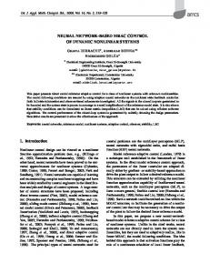
2. Face representation In order to represent faces, we use the shape representation model presented in Maggini et al. [9]. This technique exploits a set landmarks that can be extracted from an incomplete and not continuous description of the boundaries of the face parts. The landmark positions can be computed by means of Catmull-Rom splines (CRSs) [1], considering a set of non–uniformly distributed knots. Even if the initial knots are not comparable among different faces, CRSs guarantee to obtain a set of comparable landmarks. CRSs are cubic interpolating splines with a simple piecewise construction. Each segment of a CRS interpolates the curve between two knots pi and pi+1 but it is defined by four distinct knots pi−1 , pi , pi+1 , pi+2 . Given a set of n knots, with n ≥ 4, a CRS has C 1 continuity, interpolates all the points, and can exploit an unbounded number of knots to describe either closed or open curves. A change in the position of a knot does not require to recompute the whole curve. Finally, in order to obtain equally spaced landmarks along the curve, CRSs are reparameterized using arc–length parameterization [15]. Given a frontal view facial image and a set of manually labeled knots (see Figure 1a), the representation is computed ordering the knots CW or CCW, and then using CRSs to interpolate them. This leads to the description of the whole contour by means of a parametric curve. In this work, the following face parts are represented using distinct CRSs: face, nose, mouth, eyes and eyebrows (see Figure 1b). The landmarks that define this model are extracted from the CRSs that describe each part. A set of principal points (PPs) are located along each CRS using a priori knowledge on the structure of the face (see Figure 1b), and can be easily computed since they correspond to spline maxima or minima along a coordinate. Then, a set of secondary points (SPs), equally spaced between pairs of consecutive PPs, is computed (see Figure 1b). The presence of noise in a spline portion could affect the positioning of equally spaced points, but it has no effects on the other segments of the curve. An arbitrary number m of SPs between P Pi and P Pi+1 , can be computed by a uniform sampling of the spline segment bounded by the two PPs. In our work, each face is represented using 17 PPs and 32 SPs, in order to find a trade–off between the approximation accuracy and the representation compactness.

3. Learning local feature models ASMs [2] represent the shape of a face by means of a set of n landmark points, so it is particularly suited to deal with the face representation model described in Section 2. However, despite the good results achievable using ASMs to localize facial features, this technique has some limitations that are currently investigated in order to enhance its

(a)

(b)

Figure 1: Face representation: (a) Manually marked face features - (b) CRS interpolation and extraction of PPs (empty circles) and SPs (filled circles). performances. In particular, the main drawback is related to the estimation of the local feature models that are used to fit a feasible shape on an input image. In the following subsections, the traditional ASM algorithm will be briefly introduced; then, the main contributions of the AANN-ASM algorithm will be described.

3.1. Original ASMs ASMs exploit both a point distribution model (PDM), that describes the shape variability estimated on a training set, and a local feature model for each landmark, used to move the face shape across the image, in order to match the correct position. A shape is represented by a vector, containing the landmark coordinates f = (x1 , y1 , x2 , y2 , ..., xn , yn )T ∈ IR2n . In order to estimate the PDM, a training set F ∈ IR2n,m , composed by m shapes, is exploited. The shapes in F are aligned, with the aim of obtaining a common coordinate frame and a uniform size. Considering that the shapes form a gaussian distribution in IR2n , PCA is applied in order to define a generative deformable model. The mean f¯ and the covariance S of F are computed. If Φ = [Φ1 |Φ2 |...|Φc ] ∈ IR2n,c and Λ = [λ1 , λ2 , · · · , λc ]T ∈ IRc collect the c leading eigenvectors and eigenvalues of S, we can approximate a shape as f ≈ f¯ + Φb (1)

where b = Φ′ (f − f¯) ∈ IRc represents the set of parameters of the deformable model. The variance of bi , the ith entry of b, across the training set, is given by the corresponding eigenvalue λ√ i . Defining the variability range of √ bi equal to (−k λi , k λi ), being k a real valued constant (shape variability parameter), it is guaranteed that the generated shapes are similar to the examples in the training set. The shapes obtained using Eq. 1 are represented using both the coordinate frame and the scaling factor of the aligned shapes in F . As a consequence, a transformation TXt ,Yt ,s,θ (f¯ + Φb), where Xt , Yt represents a reference frame translation, s a scaling factor, and θ a rotation, must be applied to f to fit it on a given image. The face feature localization is performed generating an initial shape Y

and then analyzing the image around each landmark to find a better point position. Then, Xt , Yt , s, θ, b are updated in order to match the new position Y ′ . This process is iteratively repeated until the displacement between the positions Y and Y ′ is smaller than a certain threshold. The criterion used to find the optimal landmark position is based on a model of the local structure of the landmarks in the training set, i.e. estimating a local feature model for each landmark and looking for points that match the estimated models. For a given landmark j, let Lj = {l1j , . . . , lmj }, where lij = (xij , yij ) collects its i-th coordinate example in the training data. The set of profiles, containing 2w + 1 pixels and centered in each lij , are sampled along the normal to the shape boundary, and the modules of the luminance gradient are collected. Assuming that each sampled set is distributed as a multivariate Gaussian, the mean and the covariance are estimated to represent a statistical model for the gradient of the luminance around the landmark j. During the face feature localization, z pixels (z > w) are sampled on each side of the landmark, along the normal to the boundary. Then, at each of the 2(z − w) + 1 possible positions, the Mahalanobis distance between the sampled luminance vectors and the estimated mean model is evaluated. The position that corresponds to the lowest distance is chosen. The search is repeated for each landmark, obtaining a suggested new position Y ′ for the whole shape.

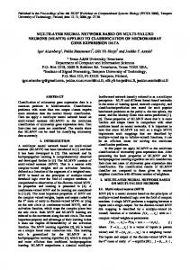
3.2. Search area estimation Given a set of landmark positions, the definition of what is considered as neighborhood and what is not, directly affects the localization performances. The sampling of some features along the normal to the boundaries leads to good results, but allowing the search to move in other directions should speed up the convergence of the algorithm. In the proposed schema, the search areas are ellipses whose dimensions depend on the training data. This choice is motivated considering that, at the end of the alignment process, the landmark positions create a set of clusters roughly centered around the mean of each group. This observation suggests to consider the landmark positions as a bivariate Gaussian distribution, that allows us to define an elliptic search area (see Figure 2a). For a given Lj , we can estimate its mean µj and its covariance matrix Σj ∈ IR2,2 . The eigenvectors Γ1 ,Γ2 of Σj correspond to the directions of the axes of the elliptic search area. The dimension of such area is determined with the aim of obtaining a region that almost always contains all the lij . If σ12 , σ22 are the distribution variances, then the ellipse defined by the two axes that goes from µj − 3σ1 Γ1 to µj + 3σ1 Γ1 and from µj − 3σ2 Γ2 to µj + 3σ2 Γ2 , covers about the 99% of the examples collected in Lj . This kind of technique allows us to statistically estimate the dimension of the seach area and to speed up the algorithm allowing movements non normal

to the face feature boundaries.

3.3. Auto Associative Neural Networks The original ASM framework uses Mahalanobis distance, in order to determine the optimal position of each landmark. However, any kind of classifier can be used to move the shape across the input image. In our work we use Auto Associative Neural Networks (AANNs), due to their proved ability to solve classification tasks, that are characterized by a well-defined class and by a “complement” class whose data are particularly heterogeneous [4, 5, 11]. Other widely used neural network models, like multilayered perceptrons, show impressive results in some applications where the data have a high inter-class and a low intra-class variability. The data involved in the prediction of a correct landmark position, however, do not satisfy such properties. In fact, the positive examples (the feasible positions) have a low intra-class variability and are quite similar among them. On the contrary, the negative examples (unfeasible positions) have, independently from the set of features used to represent the patterns, a high intra-class variability. Under this situation, standard neural network models are generally prone to misclassifications of negative examples, whereas AANNs show good generalization performances, also when processing negative examples. An AANN is a particular kind of multi-layered feedforward neural network trained to approximate the identity mapping on a subset of IRn . A non-linear AANN has usually three layers: an input layer, consisting of n units, that correspond to the components of the input vector U ∈ IRn , a hidden layer, with h < n neurons that compute their output using a non linear transfer function, and a layer of n linear output neurons. Even if AANNs are generally used for dimensionality reduction problems, they can be exploited also as classifiers. The input vector U is fed to the input units and the signals are propagated to compute the activation of the hidden and output neurons. Once the output vector O(U ) is available, the Euclidean distance ||U − O(U )|| is computed, and compared with a threshold dthr . If the output is smaller than dthr then U is classified as belonging to the positive class, otherwise it is considered as negative. The decision threshold dthr can be estimated from the distribution of the Euclidean distances obtained by processing a validation set. The AANN weights can be adapted using the BackPropagation algorithm, considering a cost function constituted by the sum of the following two contributions: Ep =

P X

||Uk − O(Uk )||2

(2)

1 ǫ + ||Uk − O(Uk )||2

(3)

k=1

En =

N X k=1

where P and N are the number of positive and negative examples, respectively. Eq. 2 measures how well the network approximates the identity mapping on the positive examples, while Eq. 3 penalizes a good approximation of the identity mapping on the N negative examples. The constant ǫ is used to prevent divisions by zero. The BackPropagation algorithm requires just a slight modification when the derivatives are computed in the case of En .

spline

α2

3.4. Set up of the learning environment α1

In order to train the AANNs we need to define both the feature set used to represent the point and the network architecture. The architecture has been chosen by a trial-anderror procedure as reported in the following section. With respect to the pattern representation, we exploit the Haarlike features defined by Viola and Jones in [14]. Such features have been chosen because their computation can be carried out in a very efficient way, exploiting integral images; moreover they produced excellent results both in face and facial feature detection problems. In particular, two, three, and four-rectangle features are computed, using four distinct resolution levels, obtaining 16 distinct features that describe each position (see [14] for further details). A positive or a negative target must be associated to each pattern in order to set up the learning environment. The choice of the target assignment policy plays a crucial role, because the presence of contradictory examples should be avoided or minimized. Assuming to know the correct landmark positions for each training image, the positive targets can be associated using information extracted from the CRSs. The splines correspond to the boundary of the face components, therefore the points that lie on the spline in a neighborhood of the true landmark position are supposed to be similar to the target point. Thus, positive examples are sampled on the part of the spline that lies inside the search area defined for each landmark. The choice of negative examples is more difficult, because we need to establish in which positions of the image the points are most likely to be different from the positive examples. Our idea is to sample the search area contour excluding the portion near the intersection with the CRS. Using this strategy, we are assured to select examples that are inside and outside the region of the considered face component, moreover, they should be dissimilar from the previously selected positive ones. Considering the angles α1 , α2 set to 20◦ , whose vertex corresponds to the landmark position, and whose bisectors pass through the intersections between the CRS and the search area contour (see Figure 2b), then we can exclude from the sampling countour the portions that lie inside α1 and α2 . The number of positive and negative examples sampled inside the search areas represents a free parameter of the proposed approach, and depends on the image complexity. Currently, the correct number of samples is determined by a trial-and-error

(a)

(b)

Figure 2: (a) Examples of estimated search areas - (b) Training point selection: positive (circle points) and negative (square points). procedure.

3.5. AANN-ASM algorithm Given the estimated PDM and the set of trained AANNs, the face feature localization proceeds as follows: 1. roughly locate the face region and place f¯ on the given image. 2. iterate the following steps: (a) for each landmark a certain number of points are sampled inside the elliptic search area and, for each point, the Haar-like features are extracted; (b) each sample is processed by the corresponding AANN and the computed distances are collected; (c) for each landmark, the coordinates of the sample corresponding to the lowest distance is choosen, and, if such distance is lower than the one associated to the current landmark position, the point is selected as the candidate for the landmark movement. (d) fit the shape to the candidate landmark positions until the convergence is reached.

4. Experimental results The proposed method has been evaluated on a subset of images extracted from the XM2VTS dataset [10], and its performances have been compared both with the results of the original ASM algorithm and with two improved versions (det-ASM and reg-ASM), recently proposed by

Cootes et al. [3]. Only faces in frontal pose and neutral expression were selected, obtaining 295 pictures (160 males, 135 females). In order to investigate the generalization capabilities of the algorithm, a 10-fold cross validation approach has been used, thus the images have been partitioned in 10 groups. Each group contains 16 males and 14 females faces (except for the last one, containing 16 males and 9 females faces). The model estimation process has been repeated 10 times, leaving out one of the subsets and using the remaining images as the training set. The shape variability parameter k was set to 2, observing that the increase of k does not allow to achieve better results. In order to perform a local search in the neighborhood of each landmark, 49 distinct AANNs were trained. Each AANN is associated to a distinct landmark. For each training image 10 positive and 10 negative examples have been extracted for each landmark, building 49 training sets. The AANNs have been trained with the standard BackPropagation algorithm, performing 10.000 training epochs. In order to choose the best network architecture, the training process was repeated several times, varying the number of hidden units between 5 and 10. The best performances have been obtained using 8 hidden units, thus the experiments described in this section are referred to this architecture. To evaluate the performances of the proposed technique, we used the mean point distance (mpd) metric, that has been computed as follows: 11X di mpd = n u i=1 n

where u is the inter-ocular distance between the eye pupils, n is the number of landmarks, di is the Euclidean distance between the i-th located point and its ground truth position. According to [3], landmarks that belong to the face boundary are excluded from this evaluation (hence n = 42) and the mpd threshold imposed to declare a successful localization has been set to 0.15. The original ASM algorithm is very sensitive to the initialization step [2]. This problem is due to the use of a limited search area, that allows a faster localization but, at the same time, avoids large movements between two consecutive iterations. Some experiments have been carried out to test the robustness of our approach. The origin of the initial model, given by the mean of the landmark coordinates, has been displaced from the true location in the 8 compass directions, by a percentage of the inter–ocular distance u. The results of the experiments, grouped by the displacement direction, are collected in Table 1. As the displacement increases the performances decrease, confirming the importance of a good initialization. Moreover, these results show that the displacement direction plays a crucial role. For southward displacements, the algorithm is most likely to converge to a good solution. This is probably due to the

Direction All NW N NE W E SW S SE

Displacement percentage 10 20 30 40 91.31 28.47 5.38 10−4 58.30 0 0 0 93.22 0.01 0 0 81.02 0 0 0 98.64 11.86 0 0 100 67.46 3.39 0 99.32 1.69 0 0 100 96.27 39.66 0.01 100 49.83 0 0

Table 1: Percentage of successful localizations obtained by AANN-ASMs varying the initial model displacement. mpd 0.06 0.08 0.10 0.12 0.14 0.15

AANN-ASM 40.3 75.6 86.7 95.6 97.3 98.6

reg-ASM 38.7 75.4 89.2 94.4 96.5 97.1

det-ASM 32.7 71.1 86.6 91.8 94.3 94.9

ASM 6.4 32.9 63.4 81.7 89.8 90.8

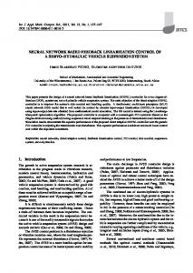
Table 2: Comparison among original ASM, det-ASM, regASM, and AANN-ASM w.r.t. their localization rate. absence of relevant edges in the lower part of the face, that makes it possible to move the shape upwards; conversely, the presence of lots of edges in the upper part (due to the presence of hair and eyebrows), makes the algorithm unable to correct a northwards initialization. In real applications we usually have no a priori knowledge on the face location, hence a preliminary detection method is needed. In order to find a bounding box containing the face, the Viola and Jones face detector has been used [14]. The experiments have been carried out initializing the origin of the initial shape model in the center of such bounding box. We experimentally evaluated that this initialization usually tends to place the starting model slightly souther of the target position, thus making the entire process more robust. As we can see in Figure 3 and in Table 2, our method outperforms both original-ASM and det-ASM, whereas it is comparable with reg-ASM. We must notice that the AANNASM curve tends to one faster than the others: we obtain a localization accuracy equal to 1, when mpd= 0.186, while reg-ASM reaches this limit when mpd≥ 1. It is important to remark that the number of landmarks that we use to represent the face parts is greater than the one exploited in [3]; the relevance of this difference on the performances will be investigated in future work. Finally, Figure 4 shows a successful localization, with

rithm. The experiments have shown promising results.

Cumulative Error Distribution

1

0.8

References

0.6

[1] E. Catmull and R. Rom. A class of local interpolating splines. Computer Aided Geometric Design, 74:317–326, 1974. [2] T. Cootes, C. Taylor, D. Cooper, and J. Graham. Active Shape Models - Their Training and Application. Computer Vision and Image Understanding, 61(1):38–59, 1995. [3] D. Cristinacce and T. Cootes. Boosted regression active shape models. In 18th British Machine Vision Conference, Warwick, UK, pages 880–889, 2007. [4] M. Gori, M. Maggini, S. Marinai, J. Sheng, and G. Soda. Edge-backpropagation for noisy logo recognition. Pattern Recognition, 36(1):103–110, 2003. [5] M. Gori and F. Scarselli. Are multilayer perceptrons adequate for pattern recognition and verification? IEEE Transactions on PAMI, 20(11):1121–1132, 1998. [6] O. Jesorsky, K. Kirchberg, R. Frischholz, et al. Robust face detection using the hausdorff distance. Proc. of Audio and Video based Person Authentication, pages 90–95, 2001. [7] A. Koschan, S. Kang, J. Paik, B. Abidi, and M. Abidi. Color active shape models for tracking non-rigid objects. Pattern Recognition Letters, 24(11):1751–1765, 2003. [8] H. Lu and W. Shi. Skin-Active Shape Model for Face Alignment. Proc. of Intl. Conf. on Computer Graphics, Imaging and Vision: New Trends, 2005, pages 187–190, 2005. [9] M. Maggini, S. Melacci, and L. Sarti. Representation of Facial Features by Catmull-Rom Splines. In Proc. of Intl. Conf. CAIP, pages 408–413. Springer, 2007. [10] K. Messer, J. Matas, J. Kittler, J. Luettin, and G. Maitre. XM2VTSDB: The extended M2VTS database. In Proc. 2nd Int. Conf. on Audio- and Video-based Biometric Person Authentication, 1999. [11] H. Schwenk. The Diabolo Classifier. Neural Computation, 10(8):2175–2200, 1998. [12] F. Sukno, S. Ordas, C. Butakoff, S. Cruz, and A. Frangi. Active Shape Models with Invariant Optimal Features: Application to Facial Analysis. IEEE Transactions on PAMI, 29(7):1105–1117, 2007. [13] B. van Ginneken, A. Frangi, J. Staal, B. ter Haar Romeny, and M. Viergever. Active shape model segmentation with optimal features. IEEE Transactions on Medical Imaging, 21(8):924–933, 2002. [14] P. Viola and M. Jones. Rapid object detection using a boosted cascade of simple features. Proc. of Intl. Conf. CVPR, 1:511– 518, 2001. [15] H. Wang, J. Kearney, and K. Atkinson. Arc-length parameterized spline curves for real-time simulation. Proc. of Intl. Conf. on Curves and Surfaces, pages 387–396, 2002. [16] Z. Zheng, J. Jiong, D. Chunjiang, X. Liu, and J. Yang. Facial feature localization based on an improved active shape model. Information Sciences, 2008.

0.4 AANN-ASM original-ASM reg-ASM det-ASM

0.2

0 0

0.05

0.1

0.15

0.2

Mean Point Distance

Figure 3: Cumulative Error Distribution [3]. Comparison among original ASM, det-ASM, reg-ASM, and AANNASM.

(a)

(b)

(c)

(d)

Figure 4: Face feature detection using AANN-ASM: (a) Initialization - (b) After one iteration - (c) After 2 iterations (d) Final result, after 6 iterations.

the intermediate results obtained at different iterations.

5. Conclusions In this paper we proposed a new technique aimed at improving the Active Shape Model algorithm. The main improvement relies on the method used to move the shape position during the localization process. A set of AANNs are trained to learn the landmark features and are exploited in order to choose the most suitable positions during the search, overcoming some limitations of the original algo-