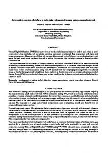
This paper describes a new method to detect features in ultrasound images, which shows ..... B. Deepak, Ultrasound Biomicroscopy, Journal of the Bombay ...
AUTOMATIC DETECTION OF FEATURES IN ULTRASOUND IMAGES OF THE EYE R.Youmaran1, P. Dicorato1, R. Munger2, T.Hall1, A. Adler1 1
School of Information Technology and Engineering (SITE), University of Ottawa, Ontario Canada
2
University of Ottawa Eye Institute, Ottawa, Ontario, Canada
ABSTRACT
In closed angled Glaucoma, fluid pressure in the eye increases because of inadequate fluid flow between the iris and the cornea. One important technique to assess patients at risk of glaucoma is to analyze ultrasound images of the eye to detect the structural changes. We propose an algorithm to automatically identify important features in the ultrasound images. Tests were performed by comparison of results with eighty images of glaucoma patients against the landmarks identified by a technologist. A success rate of 97% was achieved. This work will help improving the efficiency of clinical interpretation of ultrasound images of the eye.
Key Words: Image denoising, Region segmentation, Edge enhancement, Contrast enhancement, Feature detection, Medical imaging, Adaptive filtering, Glaucoma.
1
I.
INTRODUCTION
Glaucoma is one of the leading causes of blindness. In closed angled Glaucoma, fluid pressure in the eye increases because of inadequate fluid flow between the iris and the cornea. The pressure causes damage and eventually death of nerve fibers responsible for vision (Deepak [1]). One important technique to assess patients at risk of glaucoma is to analyze ultrasound images of the eye to detect the structural changes that reduce the flow of fluids out of the eye (Pavlin et al [2]). Usually, sequences of ultrasound images of the eye are analyzed manually; a trained technologist determines anatomical feature locations and measures the relevant clinical parameters. The main features within the eye of clinical interest are: the sclera, a dense, fibrous opaque white outer coat enclosing the eyeball except the part covered by the cornea; the scleral spur, a small triangular region in a meridional section of the sclera tissue with its base along the inner surface of the sclera; the anterior chamber, the region bounded by the posterior surface of the cornea and the central part of the lens; and, the trabecular-iris recess, the apex point between the sclera region and the iris. Manual analysis of eye images is fairly time consuming, and the accuracy of parameter measurements varies between experts. For this reason, we were motivated to develop an algorithm to automatically analyze eye ultrasound images. We anticipate that this algorithm will reduce the processing time currently taken by the technologist to analyze patient images and extract the clinical parameters of interest. The difficulties in measuring these parameters are associated with noise, poor contrast, poor resolution, and weak edge (boundary) delineation inherently present in ultrasound images (Pathak [3]). This paper describes a new method to detect features in ultrasound images, which shows good performance in detection of difficult features. The paper is organized as follows; Section II
2
presents an overview of the image processing techniques used for feature identification. Section III describes the automated algorithm for feature detection and extraction, including speckle reduction methods, non-linear contrast and edge enhancement, template correlation, region segmentation and classification, and computation of clinical parameters. Section IV presents experimental results obtained from testing the algorithm. Section V presents a discussion of previous work done in this field. Finally, Section VI concludes the paper. II.
BACKGROUND
We have found the non-linear “Log-Ratio” framework of Deng et al [4,5] to be a powerful collection of tools to sharpen edges and reduce noise in ultrasound images. This technique permits simultaneous edge and contrast enhancement while avoiding noise amplification, unlike classic techniques such as Unsharp Masking (Lim et al [6], Polesel et al [7]). We consider the image gray level digital representation in the [0,M) range, where M =256 for an 8-bit image. In order to avoid loss of information caused by intentional truncations on the processed images, arithmetic operations on image pixel values are defined in a logarithmically mapped space where the forward mapping function between the image pixel space (F) and the real number space ( ) is:
ψ ( F ) = log
(M − F ) F
(1)
Deng et al [4,5] used the symbols ⊗,⊕ and Θ to represent multiplication, addition and subtraction, respectively, in the log space. Based on this “Log-Ratio” framework, a multiscale iterative enhancement and noise reduction filter is defined as shown in Fig.1. The number of iterations depends on the high spatial frequency content of the image, as illustrated in Fig. 2. 3
After a certain number of iterations, the difference between two successive smoothed images will become very small or negligible. The enhanced image computed by the algorithm is a quasibinary image, which facilitates the selection of a threshold at the binarization process. This multiscale algorithm is designed to suppress the noise in the processed image while enhancing edges. This is achieved through selecting of the scaling parameters s. si is set to a value 1 to amplify edges and contours. Fig. 3 shows representative images of the effect of values of s. For example, Fig. 3a) illustrates an inadequate selection of the parameters (all si>1) resulting in significant noise amplification, while Fig. 3b) shows the output of the parameter values chosen in section 1.2 of this paper.
III.
ALGORITHM DESIGN This section develops an algorithm to automate the measurement of the location of
clinically relevant features in ultrasound images of the eye. The proposed algorithm is designed to calculate two clinical parameters, the open-angle and AOD 500, as shown in Fig. 4 and defined in Nishijima et al [8], and Pavlin et al [2]. In performing this calculation, it must delineate the sclera, and locate the scleral spur, the trabecular-iris recess, and the anterior chamber. The algorithm is structured into three steps, shown in Fig. 10: steps 1 and 2 are executed independently and the result merged into step 3 to complete the feature extraction and resultant calculations.
4
A. STEP 1
The goal of this section is to extract from the image the anterior chamber region. The sequences of operations are described in the flowchart (Fig. 10 a). All image operations are based on rectangular pixels of 19.5 m × 19.5 m.
1.1 Image thresholding: An intensity threshold, THR, is selected based on a subset of images of the anterior chamber region cropped manually. THR is selected at the tail of the histogram for the anterior chamber region (Fig. 5). Once obtained, THR is fixed for all scanned images. Pixels with intensity above THR are set to 255; otherwise, the value is unchanged. The thresholded image is denoted as fth1.
1.2 Non-Linear Edge & Contrast Enhancement: fth1 is low pass filtered with a 9x9 Gaussian filter with N=8 iterations, using the non-linear edge and contrast enhancement algorithm described in section II.A. The output of this system results in a coarsely enhanced image fenh1 with reduced noise and high-frequencies content. 1.3 Image Binarization: Using the grayscale threshold, THR, the quasi-binary enhanced image (fenh1) pixels are binarized (Fig. 6). 1.4 Image erosion: Erosion is applied on the binary image to remove spurious features. A 5x5 square-shaped structuring element is used for the erosion process. The resultant image is denoted by “fer1”.
5
1.5 Hole Filling: Small openings (holes) in the trabecular meshwork and the iris are detected and filled. The filled image ‘ffill1’ is later used for correlation with a template image of the anterior chamber (section 1.6). 1.6 Template Correlation: The anterior chamber is a large and roughly triangular feature, and can thus be identified using correlation with an appropriate template. In order to compensate for variability in the shape of this region, 3 template regions were chosen from representative image (Fig. 7) of subjects with different degrees of glaucoma. The enhanced image is then correlated with each template and the average correlation point (xc,yc) computed from the mean of all maximum correlation points. 1.7 Anterior Chamber Classification and Segmentation: Each closed region in “ffill1” is analyzed to identify the most likely to be the anterior chamber. Classification is based on the geometrical properties: object area, centroid, and major-axis and minor-axis length (using an elliptical model). The following parameters are computed for segmentation of each closed region: (a) Center: Defined as the center coordinate of a region (b) Distance from maximum correlation point (xc,yc): Defined as the distance between the calculated center in (a) and the average correlation point (xc,yc) computed in section 1.6. (c) Area: Defined as the total number of pixels characterizing a closed region.
The regions that meet the following requirements are to be considered as candidates in the segmentation process. (i) Area > 50 pixels; otherwise, the region is considered to be noise.
6
(ii) The distance between the center of the closed region and (xc,yc) must be minimum; ideally zero.
If more than one region has the same minimum distance, then the selection is based on the maximum area. Once the anterior chamber is segmented, the upper and lower edge coordinates are extracted. Also, the apex point (xapex, yapex) is defined by locating the black pixel that is the most to the left of the anterior chamber as shown in Fig. 4. If no regions are detected, the algorithm terminates since the coordinates of the anterior chamber cannot be calculated. B. STEP 2 The goal of this section of the algorithm is to identify the sclera region. The algorithm is shown in Fig. 10 b). 2.1 Histogram magnification: A histogram magnification (Fig. 8) is applied to enhance the texture of interest. Threshold values are calculated corresponding to 15% and 85% of the total number of pixels in the histogram. 2.2 Wiener Filtering: The image is filtered using an adaptive Wiener filter (Lim et al [6], Polesel et al [7]) with a 9x9 pixel neighborhood. The Wiener filter parameters are estimated from the local mean, variance and noise variance in an N by M neighborhood χ around each pixel.
u (χi ) =
σ 2 (χi ) =
1 NM 1 NM
f ( x, y )
(2)
( f ( x, y) − u ( χ i ) )2
(3)
x , y∈χi
x , y∈χ
The image noise variance σ N2 is defined to be the average variance for all neighborhoods. 7
1 σ = n
n
σ 2 (χi )
(4)
σ 2 − σ N2 H ( x, y ) = u + ( f ( x, y ) − u ) σ2
(5)
2 N
i =1
The filter is implemented as follows:
where H(x,y), f(x,y) are the output and input pixels, respectively. This filter adapts to the local variance as
σ 2 is
calculated for each neighborhood. Thus, if the variance is large, the filter
performs little smoothing in order to preserve high frequencies or edges. 2.3 Non-linear Edge & Contrast Enhancement: Using the same iterative process with identical parameters as in Section 1.2. 2.4 Image Binarization: Using the same process and threshold as Section 1.3, to obtain a finely enhanced binary image (Fig. 9). 2.5 Image Erosion: iterative erosion is repeated for n=4 times to remove artifacts in the enhanced binary images. The classic 3x3 erosion operator is modified in order to preserve weak edges, as follows: the center pixel (located at (0,0)) is set to background if and only if both adjacent (horizontal or vertical) pixels are background. The resultant image is denoted by “fer2”.
2.6 Region expansion: “ffill1” is dilated with a circular-shaped structuring element of size 5. This enlarges all regions in the image denoted by “fexp1”, which is used for the subtraction process described in the section 2.7.
8
2.7 Region subtraction: The expanded image (coarsely enhanced) “fexp1” is subtracted from the eroded image (finely enhanced) “fer2”. This procedure removes all large regions in the image and keeps only the fine details of interest.
2.8 Sclera region classification and segmentation: For segmentation of the sclera region, the following parameters are computed:
(a)
Boundary pixels coordinate: the pixel that is furthest to the right and is located within
each of the closed regions (xright, yright) (b)
Distance from the apex point (xapex,yapex) of the anterior chamber to (xright, yright) of each
classified region (c)
Area in pixels of each region
(d)
Major axis length of the closed regions
In order to segment the sclera from all possible regions in the enhanced image, each closed region is analyzed independently. By first scanning through the processed image, any region with an area less than 50 pixels is rejected since it is considered to be speckle noise or too small to be a proper sclera region candidate. Afterwards, the distance between (xright, yright) and (xapex, yapex) is calculated for the remaining regions with area greater than 50 and the region that has the smallest distance is considered to be the sclera.
9
If multiple regions have the same minimum distance, then the selection is based on the area and the major-axis length, based on observed ultrasound images of the eye. Once the sclera is segmented, its center (xscleral,yscleral) as well as its upper edge coordinates are extracted.
C. STEP 3
The goal of this section is to improve the robustness of the detection by applying extra fine enhancement to the original image and re-extracting a new sclera region. If the newly extracted scleral spur coordinates correlates with the one previously calculated, then the remaining clinical parameters can be computed; otherwise, the sclera region cannot be segmented, and the algorithm terminates.
3.1 Non-Linear Edge & Contrast Enhancement: The enhancement algorithm (section 2.3) is applied to feq2 computed in section 2.1. In order to achieve fine enhancement, fewer iterations (i.e. n=5) are used, resulting in a significant reduction of the blur. The enhanced image is denoted as “fenh3”.
3.2 Image Binarization: Same as in Section 1.3.
3.3 Sclera region Classification and Segmentation: The approach of section 2.8 is used except an additional parameter is used to account for the distance (dc-sc) between the center of each detected candidate region and (xscleral,yscleral). A region is classified as the best sclera candidate if it passes all the requirements of section 2.8 and has the smallest dc-sc.
10
3.4 Sclera Contour Mapping: Once the sclera has been identified (Fig. 11a), the scleral spur is located based on signal processing on the outline of the top boundary of the extracted sclera region.
This outline is determined by scanning the image vertically and determining the
uppermost location of the pixels on the sclera image (Fig.11b).
3.5 Sclera Contour Smoothing Filter Design: A non-recursive 4th order Butterworth smoothing filter, with normalized cutoff frequency (wc) of 0.45, is used to remove outliers and abrupt variations (fluctuations) in the outline that may result from poor resolution and image noise (Fig.12). The filtered data set is defined as Ffilt(x). The value of the normalized cutoff frequency was manually tuned to provide a compromise in terms shape fidelity to the shape and rejection of unwanted saddle points. Since we know that scleral spur is located to the right of the sclera region, only the right-half side of the data points on the sclera contour is searched. This truncation of the size of the detected outline reduces the search time. This new array of data is denoted as “Ftrunc(x)”.
3.6 Scleral Spur Detection: The scleral spur is detected by first applying a gradient operator on Ftrunc(x) (Fig. 11b) and then computing all minima coordinates as well as the points along the descendent edge prior to each local minimum. If no minima are detected, all points with zero gradients are located and defined as saddle edges.
Identification/detection of the scleral spur is completed when one of the following occurs:
11
If one local minimum is found, then this point becomes the scleral spur coordinate. If multiple minima are located on Ftrunc(x), then all points along the descendant edges are used in order to calculate the magnitude of each edge (∆edge) prior to a minimum. For each descendent edge found within the outline Ftrunc(x), ∆edge is computed as the difference between the maximum pixel value and the minimum pixel value along that edge. The descendant edge with the largest (∆edge) symbolizing the deepest dip is chosen as the scleral spur coordinate. On the other hand, if no minima are found along the contour, then saddle edges are used since they represent possible locations of the scleral spur on the sclera contour. Knowing a priori that the scleral spur occurs to the right side of the contour, the saddle edge located most to the right of the 1-D outline is selected as the scleral spur coordinate. The scleral spur coordinate is denoted as (xs,ys).
3.7 Determination of Measured Parameters for Glaucoma: This section describes calculation of: (1) open-angle; and (2) angle-open distance (AOD), as shown in Fig. 4.
These parameters
require the location of the apex point previously computed in section 1.7. This location will be used to define the angle.
AOD 500 & Open-Angle Calculation:
The AOD 500 is measured along an orthogonal
projection from the trabecular meshwork to the iris (Nishijima et al [8], Pavlin et al [2]), as illustrated in Fig. 4. Its calculation requires the computation of:
1) The contour along the upper half of the anterior chamber from the scleral spur to the upper vertex.
12
2) The contour from the scleral spur along the iris on the lower anterior chamber to the lower vertex. The lower contour on the processed (enhanced) image is shifted from its original location due to the blur introduced by the multiscale processing. To correct the offset imposed by the blur, we recalculate a new contour using the original image. Starting at the offset pixel position (black pixel within the anterior chamber), scan vertically in the downward direction for the first pixel that is different from black. This is shown in Fig. 13.
3) The location 500 µm from the scleral spur along the contour on the trabecular meshwork is computed using Fig. 14, as follows:
φ = tan −1
h d
(6)
y500 = y s + 25 × cos φ
(7)
x500 = x s − 25 × sin φ
(8)
where h = x s − x min and d = y min − y s The measured contours provide data for the orthogonal projection calculation between the two segments of the eye. By calculating the inner product between the vectors defined as: v1 = {( x500 − xapex ), ( y500 − yapex )} v2 (n) = {( xlower (n) − x500 ), ( ylower (n) − y500 )}
(9) (10)
we can find the orthogonal projection coordinate along the lower iris trace. n represents the sample points of the lower iris contour. Denoting this location as (xlow_mid, ylow_mid) and computing the vector
13
v3 = {( xlow _ mid − xapex ), ( ylow _ mid − y apex )}
(11)
leads to the calculation of both the AOD 500 and the open-angle. The calculation of the AOD 500 length, in µm, is given by: d AOD500 = η conv ( x500 − xlow _ mid ) 2 + ( y500 − ylow _ mid ) 2
(12)
where ηconv = 19.5 µm/pixel is the resolution of the ultrasound system used. If the 500 µm coordinate location appears to the left of the (xapex, yapex) point, then the open-angle is 0o. Otherwise, an open-angle, in radians, is calculated as:
θ = cos −1
IV.
v1 ∗ v3 v1 × v3
(13)
RESULTS
Ultrasound images were obtained from patients at the University of Ottawa Eye Institute using the Ultrasound Biomicroscopy (UBM) System Model 840 (Zeiss-Humphrey), using the protocol described in Daneshvar et al [9]. The data used within the study was taken from patients who had been diagnosed with glaucoma. The data was used initially in the study of pseudoexfoliation syndrome (Damji et al [10]). The patient’s data was then used later for this study. Patient selection was based on: 1) diagnosis of glaucoma in the patient, or 2) genetic susceptibility to the disease as indicated by its presence in their family. In total, 80 patients were enrolled in previous study. For this present work, one image was taken for each patient (in order to ensure statistical independence of results) resulting in 80 images to be analyzed. Each patient
14
was placed on a reclining chair with a headrest and an apparatus was placed surrounding the eye allowing a transducer to be placed on the ocular region. The transducer is scanned in distinct directions in order to extract the appropriate ultrasound image on the screen visible to the operator. The images are then stored on the local hard disk in PCX format. As described in Deepak [1], UBM measurements are performed with patient in a supine position with the eye open. The technologist manually identifies the location of the clinical features on the screen. The AOD 500 is then calculated and the open-angle is measured with a protractor centered at the apex point of the anterior chamber. Using the algorithm described here, 80 images were processed on a 2.4 GHz Intel Pentium III processor with 512 MB of SDRAM.
The algorithm was implemented in Matlab and the
execution time for one image is 32 seconds. In section 1.1, a threshold (THR) of 50 was used. In section 1.2, the s-parameters were set to s1,2,3,4=0.1 and s5,6,7,8 = 20 for 8 iterations. In section 2.1, the lower and upper thresholds are selected as 85 and 220, respectively. Fig. 4 illustrates all calculated clinical features of interest using this algorithm. By treating the technologist-identified parameters as gold standards, we estimated the detection position (offset) error of the algorithm. The offset error histograms are shown in Fig. 15. Overall, the offset error was smaller in the vertical direction compared to the horizontal direction. In the horizontal direction, the mean error is 2 pixels (39.5 mm) toward the eye center and standard deviation is calculated to 6.7 pixels (130.65 mm). In the vertical direction, the mean error is 1.42 pixels (27.69 mm) toward the back of the eye with a standard deviation of 2.71 pixels (52.8mm).
15
Three possible outcomes can be generated by the developed algorithm. If the algorithm fails to segment the regions of interest or cannot process a specific image, the clinical parameters are not computed (outcome 1). Otherwise, clinical parameters are computed. If the calculated parameters differ from those measured by the technologist within 97.5 um (5 pixels), the output is considered a success (outcome 2). Otherwise, the offset error is greater than 97.5 um (5 pixels) in both direction, and the algorithm output is a failure (outcome 3). Based on the outcomes described above, in 5% of cases, the algorithm could not analyze the images (outcome 1). In the remaining cases where clinical parameters are computed, features were correctly identified in 97% of images (outcome 2). Thus, 3% of images presented inaccurate estimates (outcome 3) of the clinical parameters, with 351 um (18 pixels) offset error average. Fig. 16 shows an ultrasound image of the eye with all clinical parameters computed successfully (outcome 2).
V.
DISCUSSION
This paper has developed an algorithm to automatically identify features in ultrasound images of the eye and compute the clinical parameters of interest to the technologist. Many algorithms have been proposed in order to enhance and detect features in ultrasound images. The algorithms chosen in this work were those found experimentally to give good results. In developing this work, several different approaches were tested in order to select the approach presented in section III. Based on the results obtained from testing the developed method on
16
sample images, we believe that the accuracy of the algorithm can be further improved by adjusting the saddle and minima locator technique described in section 3.6. Because of the large body of work on ultrasound image processing algorithms, we feel that it is valuable to provide briefly review and comment on the applicability of these algorithms to the problem considered in this paper. Recently, there has been active research on image denoising and speckle reduction in ultrasound and Synthetic Aperture Radar (SAR) images. In Xie et al [11] a spatially adaptive noise reduction algorithm is constructed for image denoising using a combination of wavelet Bayesian methods and a Markov random fields image regularization technique. In Ulfarsson et al [12] a speckle-reduction algorithm is proposed in the Curvelet domain where a threshold is applied on the coefficients for the denoising process. In Saevarsson et al [13] a fusion of the undecimated discrete wavelet transforms (UDWT) and a time invariant discrete curvelet transform (TIDCT) is used for speckle-reduction in SAR images. These methods perform well for image denoising but to achieve proper texture segmentation in ultrasound images, additional edge enhancement techniques should be applied. Many other techniques exist for ultrasound image denoising. For example (Xie et al [11], Ulfarsson et al [12], Saevarsson et al [13]) are based on processing in wavelet domain where the selection of a wavelet mother basis depends on the application. These techniques focused uniquely on speckle reduction. In Zong et al [14], a speckle reduction and contrast enhancement in the wavelet domain was proposed. The noise reduction was obtained by soft thresholding the wavelet coefficients and feature enhancement was accomplished via nonlinear stretching followed by hard thresholding of wavelet coefficients within selected spatial-frequency levels.
17
The technique showed good results for visual image improvement, but feature identification and segmentation were not explored. Also, wavelet coefficients thresholding leads to the appearance of parasitic oscillations in the vicinity of edges. In Bezvesilniy et al [15], a wavelet-based image processing, edge detection and noise reduction technique is proposed. This method overcomes the oscillation problem by using a first derivative of the cubic B-spline as the analyzing wavelet. This led to well-behaved edge representation in the wavelet domain where edges are sharp and well localized and do not have oscillations. This approach also allows edge classification and processing based on edge height. However, this approach may not be stable in the presence of ultrasound speckle noise. This is because texture analysis in ultrasound images is difficult, especially in an application such as this, due to the poor boundary delineation near the sclera tissue. Other existing methods that combine denoising, enhancement and feature detection of ultrasound images include the use of Gabor filter texture segmentation (Xie et al [17]) and diffusion filter and sticks (Pathak et al [3]). In Mohamed et al [16], the spatial parameters of the Gabor filter are tuned and applied to Trans-rectal ultrasound images of the prostate (TRUS) such that the filter output magnitude matches the desired texture.
The outline of a cancerous region is then
segmented by providing the algorithm some texture information. In order to capture all texture areas, large filter banks are required to analyze the image. In Xie et al [17], a method for kidney segmentation based on texture analysis by applying a bank of Gabor filters was developed to process the ultrasound image, based on proper modeling of shape priors for segmentation. In this technique, the initial segmenting curves were positioned manually requiring the input of trained users for each image.
18
Another approach in ultrasound defines line segments called sticks (Pathak et al [3]) in different angular orientations as templates that model false edges while reducing speckle. The technique allows contrast enhancement only at the edges, while noise is decreased.
An anisotropic
diffusion filter is used to further smooth the image and reduces noise to allow for Canny edge detection. The method allows a technician to overlay the detected edges on the original image to assist manual delineation of the prostate. The methods reviewed can be generally used to process the ultrasound images. However, fully automated techniques were not developed to detect and extract the areas of interest, which was our main objective in this paper.
VI.
CONCLUSION
This paper proposes an algorithm to automatically identify clinical features in ultrasound images of the eye. The algorithm computes the AOD 500 and the open-angle parameters used to measure the presence and severity of glaucoma. Overall, the algorithm predictions are very similar to the trained technologist’s observation with a small (±0.1mm) pixel offset error in both the horizontal and vertical directions. In the processed images, features were correctly identified in 97% of the cases. 3% of images presented inaccurate approximation of the clinical parameters, with 351 um error average. The difficulties encountered in measuring clinical parameters are associated with the speckle noise, poor contrast, poor resolution, and weak edge delineation present in the processed ultrasound images. These issues introduced inaccuracy in locating the scleral spur and variability in the measurement of the clinical parameters. The algorithm was designed with a goal of robustness through the use of two-stage (coarse and fine) level enhancement on the original image, and by validation of the proper segmentation of the sclera at
19
each step. Overall, the benefit of this work is the ability of algorithm to reduce the processing time and improve processing consistency for each patient’s ultrasound image, leading hopefully to an increase in efficiency and a reduction of cost.
20
REFERENCES 1. B. Deepak, Ultrasound Biomicroscopy, Journal of the Bombay Ophthalmologists Association 12, 1-4 (2002). 2. C.J. Pavlin, K. Harasiewicz, M.D. Sherar, F.S. Foster, Clinical Use of Ultrasound Biomicroscopy, Ophthalmology 98, 287-295 (1991). 3. S.D. Pathak, V. Chalana, D.R. Haynor, Y. Kim, Edge-Guided Boundary Delineation in Prostate Ultrasound Images, IEEE Transactions on Medical Imaging 19, 1211-1219 (2000). 4. G. Deng, L.W. Cahill, Image Enhancement Using the Log-ratio Approach, Signals Systems and Computers 1, 198-202 (1994). 5. G. Deng, L.W. Cahill, Multiscale image enhancement using the logarithmic image processing model, Electronics Letters 29, 803-804 (1993). 6. J.S. Lim, Two-dimensional Signal and Image processing, Englewoods Cliffs, NJ: PrenticeHall, 536-540 (1990). 7. A. Polesel, G. Ramponi, V.J. Mathews, Adaptive unsharp masking for contrast enhancement, Image Processing Proceedings 1, 267 – 270 (1997) 8. K. Nishijima, K. Takahashi, R. Yamakawa, Ultrasound Biomicroscopy of the Anterior Segment after Congenital Cataract Surgery, American Journal of Ophthalmology 130, 4 (2000). 9. H. Daneshvar, S. Brownstein, G. Mintsioulis, D. Chialant, K. Punja, K.F. Damji, Epithelial ingrowth following penetrating keratoplasty:A Clinical, Ultrasound Biomicroscopic and Histopathological Correlation, Canadian Journal of Ophthalmology 35, 222-224 (2000). 10. K.F. Damji, H.S. Bains, E. Stefansson, Is pseudoexfoliation syndrome inherited? A review of genetic and nongenetic factors and a new observation, Ophthalmic Genetics 19, 175-185 (1998).
21
11. H. Xie, L.E. Pierce, F.T. Ulaby, SAR Speckle Reduction Using Wavelet Denoising and Markov Random Field Modeling, IEEE Transactions on Image processing 40, 2196-2212 (2002). 12. M.O. Ulfarsson, J.R. Sveinsson, J.A. Benediktsson, Speckle reduction of SAR Images in the Curvelet Domain, Proceedings of the International Geoscience and Remote Sensing (IGARSS) 1, 315-317 (2002) 13. B.B. Saevarsson, J.R. Sveinsson, J.A. Benediktsson, Combined Wavelet and Curvelet Denoising of SAR Images, Proceedings of the International Geoscience and Remote Sensing Symposium (IGARSS) 6, 4235 – 4238 (2004) 14. X. Zong, A.F. Laine, E.A. Geiser, Speckle reduction and contrast enhancement of echocardiograms via multiscale nonlinear processing, IEEE Transactions on Medical Imaging 17, 532 - 540 (1998). 15. O. Bezvesilniy, V. Vinogradov, D. Vavriv, K. Schunemann, Wavelet-based image processing: edge detection and noise reduction, 17th International Conference on Applied Electromagnetics and Communications 1-3, 123 – 126 (2003). 16. S.S. Mohamed, T.K. Abdel-galil, M.M.A.Salama, A.Fenster, D.B. Downey, and K. Rizkalla, E.F. El-saadany, M. Karnel, Prostate Cancer Diagnosis Based on Gabor Filter Texture Segmentation on Ultrasound Image, IEEE CCECE, 1485–1488 (2003). 17. J. Xie, Y. Jiang, H. Tsui, Segmentation of kidney from ultrasound images based on texture and shape priors, IEEE Transactions on Medical Imaging 24, 45 – 57 (2005).
22
FIGURES:
Figure 1
(a)
(b)
(c)
(d)
(e)
Figure 2
Figure 3
23
Figure 4
Figure 5
Figure 6 24
Figure 7
Figure 8
Figure 9
25
Step 1
Step 2
C oarse ehancem ent an d Anterior cham ber segm en tation
Step 3
Fin e eh ancem ent and sclera segm entation
E xtra fine ehancem ent and clinical param eters com p utation
O riginal Im age f(x,y ) 2.1 Histogram
3.1 E dge & C o ntrast enhancem en t ([9 9] G aussian PS F , N=5)
M agn ification
f eq2 1.1 Im age th resholding
2.2 W iener LPF
f th1 1.2 E dge & C on trast en hancem ent ([9 9] G aussian PS F , N=8)
2.3 E dge & C ontrast enhancem ent ([9 9] G aussian PS F , N=8)
1.5 Hole filling
2.4 Im ag e Binarization
2.6 R eg ion expansion
f exp1
3.4 C ontour m ap
3.5 Bu tterworth LPF
2.5 Im age E rosion
-
f er2
S earch for M inim a?
No
f fill1 1.6 T em plate co rrelation
3.3 R esegm entation of sclera
f enh2
1.3 Im age Binariz ation
f er1
3.2 Im age Binariz ation
f sm 2
f enh1
1.4 Im age E rosion
f enh3
2.8 R eg ion classification and S egm entation {extract (xscleral, y scleral)}
Y es
Locate saddle edg e to the right
1.7 R egion classification and S eg m entation
C alculate descen dant edges
F ind S ad dle ed ges
No
> T hreshold
Y es Pick m inim a w ith deepest ed ge
3.6 Find S cleral p oint
3.7 C alcu lation of openin g angle and AO D 500
Figure 10
26
(a)
(b) Figure 11
27
Figure 12
Figure 13
28
(x500, y500) (xs, ys)
(xmin, ymin) h
φ
d (xmax, ymax)
Figure 14
(a)
(b) Figure 15
29
Figure 16
30