COST OPTIMIZATION OF SLAB MILLING OPERATION USING GENETIC ALGORITHMS Bhavsar, S.N. and Sanghvi, R.C. G H Patel College of Engineering and Technology, Vallabh Vidyanagar – 388 120, Anand, Gujarat E-mail:
[email protected];
[email protected] Abstract In order to optimize the objective function for machining, one needs to determine cutting parameters, such as speed, feed and depth of cut. Here, it is presented the use of Genetic Algorithms (GAs) to minimize the cost for slab milling operation on horizontal milling machine. The depth of cut and feed values are set to suit the machine condition and surface finish requirements, while cutting velocity is optimized for minimum cost of production. A correction factor is incorporated to GAs for correcting the results of optimum cutting speed and optimum cost of production. At the end the cost optimum cutting speed and optimum cost generated by GAs are compared with the results generated by traditional optimization method of using Taylor’s equation of tool life, for its validation. Comparison of results evolves the efficiency of GAs for finding the cost optimum cutting parameters. Keywords: Genetic Algorithms, Slab Milling, Cost Optimization. 1. INTRODUCTION Of vital interest to the manufacturing engineer are production cost and production rates. Although, in practice a high production rate would probably mean low production costs, it should be pointed out that these two factors must be considered separately and that the manufacturing conditions giving maximum production rate will not be identical to those conditions giving minimum cost of production. The machining economics problem (shaw, M.C.; Lissaman, A.J. and Martin, E.J.; Chapman, P.C.) consists in determining the process parameters, usually the cutting speed, feed rate and the depth of cut, in order to optimize the objective function. Moreover, in determining these parameters, special attention is usually given to the restrictions or the constraints imposed on the particular operation by the machine tool, the cutting tool and the work piece. For the purposes of the discussion it is necessary to explain that feed is the distance moved by the tool relative to the work piece in the feed direction for each revolution of the tool or the work piece or each stroke of the tool or work piece. Confusion may arise in certain multipoint tool operations, such as milling, where the feed setting on the machine refer to the relative speed between the tool axis and the work piece in the feed direction (the feed speed). Thus, if the feed speed in the milling operation is vf and the rotational frequency of the tool is nt, the work piece feed during each revolution of the cutter is given by vf / nt, and the maximum cutting speed v in a milling operation is given by πdtnt, where dt is the tool diameter. It now follows that if it is required to double the cutting speed in a milling operation while keeping the feed constant, it would be necessary to double both the rotational frequency of the cutter nt and the feed speed vf (Boothroyd, G.). A number of machining optimization approaches have been reported, some of these approaches were limited to single pass operations (Wang, J. et al.; Kirov, K.P. and Hristov, H.I.). The parameters usually optimized in a single pass are the cutting speed and the feed rate. The other approaches considered the multi pass operations (Sonmet, A.I. et al.; Onwubolu, G.C. and Kumalo, T.; Amiolemhen, P.E. and Ibhadode, A.O.A.). In the multi pass operations, the parameters to be optimized are the depth of cut or the number of pass, the cutting speed and the feed rate. Onwubolu et al. shows that Genetic Algorithms (GAs) is most suitable for the optimization of machining parameters. Simulated Annealing is also used to find out the optimum machining parameters in multi pass operations (Saravanan, R. et al.). In this work slab milling operation is selected for single pass operation. GAs were applied to find out the cutting velocity, which gives minimum cost of production for given feed rate and depth of cut. At the same time the results of optimization generated by GA are compared with the results obtained by routine analytical method of optimization which uses Taylor’s equation of optimum tool life. 2. ROUTINE METHOD OF COST OPTIMIZATION 2.1 Choice of Feed
1
It is known that the correct feed to use in roughing operations is the highest the machine tool can withstand in terms of tool forces and power consumption. When a finishing cut is to be taken, the appropriate feed will be that which will give an acceptable surface finish. 2.2 Choice of Cutting Speed 2.2.1 Taylor’s Equation for Choice of Cutting Speed In choosing the cutting speed for a machining operation, we shall follow the approach described by Boothroyd, G. Here, the time spent by the operator and his machine in producing a batch of components Nb can be separated into three items: 1. The nonproductive time, given by N b t l , where t l is the time taken to load and unload each 2.
component and to return the tool to the beginning of the cut. The total machining time, given by N b t m , where t m is the machining time for the component.
3.
The time involved in changing worn tools, given by N t t ct , where and
t ct is the tool changing time,
N t is the number of tools used.
Thus, if M is the total machine and operator rate (including overheads), the total machine and operator costs will be (1) M ( N b t l + N b t m + N t t ct ) To this cost, must be added the cost of the tools used, given by N t C t , where
C t is the cost of each
tool. The average production cost Cpr for each component can now be written
C pr = M t l + M t m + M
Nt N t ct + t C t Nb Nb
(2)
The first item in the expression is the nonproductive cost, which is constant for the particular operation. The second item is the machining cost, which is reduced as the cutting speed is increased at constant feed. The final items are the tool costs, which increase as the cutting speed increases. To calculate the number of tools used in producing the batch of components, it is necessary to know the relationship between the cutting speed and tool life. The work of Taylor showed that an empirical relationship exists between these variables, namely, n
v tr (3) = v t r where v = cutting speed, t = tool life, n = constant, t r = measured tool life for a cutting speed v r . The value of t r may be found for a particular work piece and tool material and a particular feed either by experiment or from published empirical data. The index n depends mainly on tool material; for high speed steel n ≅ 0.125, for carbide 0.25 < n < 0.3, and for ceramics 0.5 < n < 0.7. Figure 1 gives the approximate ranges for the values of v r for various tool and work materials when the tool life is 60s. The tool life t for a particular situation is therefore given by
v t = tr r v
1
n
(4)
It should be noted that, traditionally, the Taylor tool life equation has been applied in the form
vtn = C The number of tools
(5)
N t used in machining the batch of components is given by N b t m / t assuming
that the tool is engaged with the work piece during the entire machining time. Thus,
N t tm tm v = = Nb t t r vr
1
n
Finally, the machining time for one component is given by
tm =
K v
(7)
2
(6)
Fig. 1. Approximate values of the cutting speed
v r when tool life t r = 60 sec (Boothroyd, G.)
where v is the cutting speed and K is a constant for the particular operation. In slab milling operation, the value of K will be given by π d l / f , where l is the length to be traveled by cutter, d is the diameter of the cutter and f is the feed. The relationship between the production cost and the cutting speed can now be obtained by substitution of equations ( 6 ) and ( 7 ) in equation ( 2 ):
C pr = M t l + M To find the cutting speed
(1− n ) K K + 1 (M t ct + Ct ) v n v v nt r r
(8)
vc for minimum cost, equation ( 8 ) must now be differentiated with respect
to v and equated to zero. Thus
n M tr vc = v r 1 − n M t ct + C t
n
(9)
2.2.2 Tool Life Determination In analyzing practical machining operations it is convenient to employ expression for the optimum tool life for minimum cost t c . This expression can be obtained by substitution of equation ( 9 ) in Taylor’s tool life equation ( 4 ). Thus,
tc =
C 1− n t ct + t n M
( 10 )
Finally the corresponding optimum cutting speeds can be found from
3
t vc = v r r Q tc
n
( 11 )
The value of Q for slab milling can be obtained from geometries shown in figure 2. Thus for slab milling,
Q= where
2a 1 1 θ = + arcsin e − 1 2π 4 2π dt
( 12 )
a e is the working engagement and d t is the tool diameter.
3. Genetic Algorithms (GAs) Philosophically, GAs are based on Darvin’s theory of survival of the fittest. GAs are based on the principles of natural genetics and natural selection. The basic elements of natural genetics – reproduction, cross over, and mutation – are used in the genetic search procedure (Rao, S.S.) Initially a population of points is used for starting the procedure instead of a single design point. Reproduction is a process in which the individuals from initial population are selected based on their fitness values relative to that of the population. In this process each individual string is assigned a probability of being selected for copying. Thus individuals with higher fitness values have greater chance of being selected for mating and subsequent genetic action. Consequently, highly fit individuals live and reproduce, and less fit individuals die. After reproduction, the cross over operation is implemented in two steps. First, two individual strings are selected at random from the mating pool generated by the reproduction operator. Next, a cross over site is selected at random along the string length, and the binary digits are swept between the two strings following the cross over site. The new strings obtained from the cross over (off-springs) are placed in the new population and the process is continued. Finally, a mutation operator is applied to the new string with a specified mutation probability. A mutation is the occasional random alteration of a binary digit. Thus, I mutation a 0 is changed to 1, and vice versa, at a random location. 4. Implementation The procedure explained in section 3 for GAs is implemented in C++ language for the following cutting conditions on a Horizontal Milling machine for slab milling operation. 2 Work piece Material = Cast Iron ( Tensile Strength = 425 MN/m ) Cutting Tool Material = High Speed Steel Cutter Diameter, d = 0.050 m Length of Work piece = 0.1 m Length to be Traveled by Cutter, l = 0.15 m Feed Rate, f = 0.01 mm/rev
M = Rs. 4/- per min t l = 180 sec t r = 60 sec (figure 1) t ct = 300 sec v r = 3.5 m/s (figure 1) C t = Rs. 100/- per cutting tool n = 0.125
4
Fig. 2. Slab milling operation According to the machine tolerable limit and surface roughness requirements, values of depth of cut and feed rate have been selected for machining. Here cutting speed is required to be optimized for the operation mentioned above. The Genetic Algorithms is planned to take initial population of ten different speed values from the range of 1 rpm to 4095 rpm. For this purpose a total of 12 digit binary 11 number is generated for each speed selected in a generation, i.e. 2 . After getting the values of cutting speeds, we need to calculate the total cost of production for individuals ( fx (i ) ) with the help of equation (8). As GAs are used to obtain the maximum value, our problem is converted to maximization by subtracting each cost value from the maximum cost value and gives difference of costs for ten speed values ( f 1(i ) ) . Now to find out probability of individual cutting speeds, each
( f 1(i ) )
is divided by
∑ f 1(i) . The cumulative probability is determined for reproduction from the
initial population. Two point cross over operator is applied on this reproduction pool for swapping the strings. Afterwards the strings are mutated with probability of 0.05. This completes one generation. Table 1 shows the result of sixth generation. Table2 shows the optimum result of each generation. The values of velocity in table2 does not consider the effect of parameter Q = 0.14 (Boothroyd, G.), which must be considered for slab milling operation according to equation (11). Hence the corrected optimum velocity from table2 is,
1.8003 1.8003 = = 2.3019 m/s Qn 0.14 0.125 Now the corrected minimum cost can be calculated by putting this value of cutting velocity in equation (8), which is 151.9033 Rs.
Sr. No.
1 2 3 4 5 6 7 8 9 10
Binary Values of Speed
011010111110 000001110110 000010111110 001011100110 001011100110 001011100110 001010111110 001010111101 011001111110 011011100110
Speed RPM
1726 118 190 742 742 742 702 701 1662 1766
fx (i)
Cost difference
Rs
f 1(i )
8067.647 520.733 727.951 114.669 114.669 114.669 112.281 112.256 6204.885 9462.078
Rs 1394.431 8941.346 9134.127 9347.409 9347.409 9347.409 9349.798 9349.822 3257.193 0.000
Cost
Prob.
Cum. Prob.
Random No.
String No.
No. of Strings
0.02 0.13 0.13 0.13 0.13 0.13 0.13 0.13 0.05 0.00
0.02 0.15 0.28 0.41 0.55 0.68 0.82 0.95 1.00 1.00
0.48 0.17 0.54 0.49 0.87 0.68 0.34 0.51 0.66 0.85
5 3 5 5 8 6 4 5 6 8
0 0 1 1 4 2 0 2 0 0
Table 1. GAs Result At Sixth Generation Sr. No.
Population after Reproduction
String no. for Cross
1st site of Cross
2nd site of Cross
5
Result of Cross over
Result of Mutation
1 2 3 4 5 6 7 8 9 10
000010111110 001011100110 001011100110 001011100110 001011100110 001011100110 001011100110 001011100110 001010111101 001010111101
Generation No. 1 2 3 4 5 6 7 8 9 10
over 8 4 9 2 6 5 10 1 3 7
Minimum Cost Rs. 2491.407 113.654 113.654 112.281 112.181 112.256 112.256 112.256 112.256 112.256
over 2 5 1 5 8 8 10 2 1 10
over 6 9 3 9 9 9 11 6 3 11
001011111110 001011100110 001011100110 001011100110 001011100110 001011100110 001011100100 000010100110 001010111101 001010111111
Table 1. Continued Velocity Generation m/s No. 3.8099 11 1.6694 12 1.6694 13 1.8369 14 1.8369 15 1.8343 16 1.8343 17 1.8343 18 1.8343 19 1.8343 20
Minimum Cost Rs. 112.256 112.116 112.116 112.116 112.116 112.116 112.116 112.116 112.116 112.078
001011111110 011011000110 001001100110 001011100110 001011100110 001011100110 001011100100 000011100110 000010111101 101010111111
Velocity m/s 1.8343 1.7741 1.7741 1.7741 1.7741 1.7741 1.7741 1.7741 1.7741 1.8003
Table 2. Results of Twenty Generations If we follow the routine method of optimization with Taylor’s equation, then first we need to determine t c from equation (10). This is the optimum tool life for cost minimization. Now from equation (11) calculate vc , which is the optimum cutting velocity for cost minimization. This value of cutting velocity gives the minimum production cost when substituted in equation (8). The values calculated with the help of Taylor’s equation are as follows, which can be compared with the result of Genetic Algorithms.
t c =12,600 sec vc = 2.2936 m / s C pr = 150.3676 Rs. 5. Conclusion Difficulties arise when the optimization process involves many parameters that interact in highly nonlinear way. In this situation number of constraints over the problem may also be quite high. These kind of problems can be efficiently solved by heuristic methods like Genetic Algorithms and Simulated Annealing. 6. References Amiolemhen, P. E. and Ibhadode, A. O. A. (2004). Application of Genetic Algorithms – determination of the optimal machining parameters in the conversion of a cylindrical bar stock into a continuous finished profile. International Journal of Machine Tools and Manufacture, 44, 1403 - 1412. Boohroyd, G. (1985). Fundamentals of metal machining and machine tools. McGraw-Hill Book Company Inc. Chapman, P. C. (2002). Production engineering technology. Tata McGraw-Hill Publishing Company Limited. Kirov, K. P. and Hristov, H. I. (2002). System for cutting conditions optimization of machining. Trakya Universitesi bilimsel alastrirmalar Dergisi B. serisi Cilt 3(2), 149-154. Lissaman, A. J. and Martin, E. J. (1972). Principles of engineering production. The English Universities Press Limited, London.
6
Onwubolu, G. C. and Kumalo, T. (2002). Multi pass turning optimization based on Genetic Algorithms. International Journal of Production Research, 39(16), 3727-3745. Rao, S. S. (1996). Engineering optimization : theory and practice. New Age International (P) Limited, New delhi. Saravanan, R. et al. (2003). Machining parameters optimization for turning cylindrical stock into a continued fiished profile using Genetic Algorithms and Simulated Annealing. International Journal of Advance Manufacturing Technology, 21, 1-9. Shaw, M. C. (1999). Metal cutting principles. CBS Publishers and Distributors, New Delhi. Sonmez, A. I. et al. (1998). Dynamic optimization of multi pass milling operation via geometric programming. International Journal of Machine Tools and Manufacture, 39, 297-320. Wang, J. et al. (2002). Optimization of cutting conditions for single pass turning operations using a deterministic approach. International Journal of Machine Tools and Manufacture, 42, 1023-1033.
7