1 2 3 4 5 6 7 8 9 10 11 12 13 14 15 16 17 18 19 20 21 22 23 24 25 26
Developing a Methodology for Social Network Sampling D. W. Franks1*, R. James2, J. Noble3, and G. D. Ruxton4 1
York Centre for Complex Systems Analysis, Department of Biology & Department of Computer Science, University of York, YO10 5YW 2 Department of Physics & Centre for Mathematical Biology, University of Bath 3 Science and Engineering of Natural Systems Group, School of Electronics and Computer Science, University of Southampton 4 Division of Environmental & Evolutionary Biology, Institute of Biomedical and Life Sciences, University of Glasgow
Abstract Researchers are increasingly turning to network theory to understand the social nature of animal populations. We present a computational framework that is the first step in a series of works that will allow us to develop a qualitative theory of social network sampling to aid ecologists in their social network data collection. To develop our methodology, we need to be able to generate networks from which to sample. Ideally, we need to perform a systematic study of sampling protocols on different known network structures. Thus, our aim here is instead to develop a computational tool for generating network structures that have userdefined distributions for network properties and for key measures of interest to ecologists. The user defines the values of these measures and the tool will generate appropriate network randomizations with those properties. We describe the method used by the tool, demonstrate its effectiveness and discuss how the tool can now be utilised.
*
Corresponding author: Email:
[email protected]. Tel: 01904 328648
1
1 2 3 4 5 6 7 8 9 10 11 12 13 14 15 16 17 18 19 20 21 22 23 24 25 26 27 28 29 30 31 32 33 34 35 36 37 38 39 40 41 42 43 44 45 46 47 48 49 50
Introduction Researchers are increasingly turning to network theory to understand the social nature of animal populations (e.g., Croft et al. 2004, Lusseau and Newman 2004, Sibbald et al. 2005). Network theory (or graph theory) offers a powerful set of statistical measures that allow us to quantify, describe and compare the structure of social relations. To make use of these measures, ecologists need to gather relational data (for example, lists of observed associations) regarding the social relations of the study species. These relational data are typically collected by sampling the social relations through observing the animals over a given time-period. Thus, due to effort constraints and the practical difficulty involved in tracking animals, these sampled relational data produced are usually a subset of the actual network. Once the sample of network data has been collected ecologists can perform a statistical network analysis. Key measures of a social network that ecologists often quote are: average degree (the average number of connections of each node), average path length (the average number of intermediate nodes between any two nodes), clustering (the probability that two nodes with a mutual neighbour are themselves connected), betweenness (the extent to which a given node acts as a ‘broker’ between other nodes) and assortativity (whether social connections are linked to another trait of interest, such as sex or age). There are many more useful measures that can be taken (Wasserman et al. 1994). Ecologists take these measures of the sample as informative of the structure of the real-world animal social structure. In other words, the assumption is that the sampled social network is structurally equivalent to the actual social network. If this assumption does not hold, then the statistical properties of the sampled network will be uninformative (and potentially misleading) as to the social structure of the animal population. We need to have confidence, then, that our sampled network does not give artefactual statistical properties caused by sampling biases. The various network measures taken on the sample may be biased estimators of the true values. For example, just as we will get a biased estimate of mean human height by selecting for our sample those people who stood out in a crowd, we will get a biased estimate of a measure like mean connectivity if we sample individuals who are socially prominent. This is a significant problem given that a qualitative theory of ecological network sampling is currently considerably lacking (but for some preliminary work, often with application to other areas of research see, Costenbader and Valente 2003, Borgatti et al. 2006, Kossinets 2006, Lee et al. 2006, Yoon et al. 2007). There are many sampling questions we can ask such as: What proportion of the whole network needs to be observed to provide us with accurate network measures? For how long do samples need to be taken? What type of sampling works best for different social behaviours? What sampling protocol is best for the system in question? How can we make best use of limited effort? Here, we take the fist step in developing a qualitative methodology of social network sampling to aid ecologists in their data collection. The sampling theory should be practical, and take into consideration limitations on resources, effort, and the ability to track animals. We are, in any case, unlikely to gain perfect samples. Our analysis will therefore need to examine the tradeoff between effort and sample accuracy. To illustrate how effort constraints might affect the sampled network’s fidelity let us consider the snowball sampling technique. Snowball sampling is an ego-centric technique for building a sample network spanning out from select individuals (Frank 1979). First, individuals are initially selected at random from the same geographical region and their social relations are
2
1 2 3 4 5 6 7 8 9 10 11
recorded over a number of time-steps. Then, all neighbours of the previous focal individuals are selected as new focal individuals and their connections are recorded. The process is repeated until the researcher decides that a large enough network sample has been taken. This creates a complete sub-network centred around the initial focal individuals. Snowball sampling can be impractical due to the excessive resources required for keeping track of (or reliably re-finding) a large number of individuals. Thus, it might be easier to employ a kind of quasi-snowball sampling to the data collection. This quasi-snowball sampling might involve limiting the number of individuals followed in each stage. At the extreme, only a single individual might be followed. What are the implications of modifying the snowball sampling technique? We need to develop a quantitative study to find out. 64 95 0
45
9
26 13
51
78 56
90 61
31
59
80 29
84 86
39
47 28
89
66
15
70
36
3
37
14 82
21
67
83
52
17 88
53
16
20
33
32
5
94
43
1
25
7
65
93
49
4
71
63 74
62
92
40 34
85
72
50 22
18
76
96
8
42
10 73 23 99
6
44
24 2
69
57 97
12
91
30
41
58
27
68
87
55 35
46
81 77
11
79
98 75 54
38
12 13 14 15
19
48 60
Figure 1: A random network with 100 nodes, a mean degree of 3, an average path length of 4.46, a degree correlation of -0.01, and a clustering coefficient of 0.02. Numbers next to each node are simply node identifiers.
16 75
94
25
45
30
40 9
13 80
12
31 24
91
97
62 88
90
35
41
96
68
8
57
59 53
92
63
23
69
32 34 1
10
20
81 77
36
33 16
49
79
84 73 61
52 54
19 85
17 18 19 20 21 22 23
Figure 2: A network constructed using quasi-snowball sampling (see text for description) from the random network shown in figure 1. Numbers next to each node are node identifiers. The sampling arbitrarily started at node 53 and stopped after 30 individuals had been tracked. The red nodes have been sampled, and the white nodes have been observed interacting with a sampled individual, but have not been directly sampled themselves. This sampled network has 30 nodes, a mean degree of 2.34, an average path length of 4.79, a degree correlation of -0.39, and a clustering coefficient of 0.04.
24
3
1 2 3 4 5 6 7 8 9 10 11 12 13 14 15 16 17 18 19 20 21 22 23 24 25 26 27 28 29 30 31 32 33 34 35 36 37 38 39 40 41 42 43 44 45 46 47 48 49 50
To demonstrate potential problems of biased sampling we give a single example of simulating sampling from a network. This is only a single example and is intended for demonstration purposes only; it is not part of our quantitative sampling theory. Figure 1 shows a random network with 100 nodes, a mean degree of 3, an average path length of 4.46, a degree correlation of -0.01, and a clustering coefficient of 0.02. The degree correlation (or assortativity coefficient) is the Pearson correlation coefficient between connected pairs of nodes (formally defined in, Newman, 2002). This gives a number that is positive for assortative mixing (positive degree correlation) and negative for disassortative mixing (negative degree correlation). Essentially, assortative mixing is a preference for high-degree vertices to attach to other high-degree vertices, while disassortative mixing is a preference for high-degree vertices and low-degree vertices to attach. Ecologists might be interested in the degree correlation if they are examining, for example, the transmission of information, or spread of a virus, throughout the network. Assortative mixing by degree would suggest that well-connected individuals have a tendency to relate to other well-connected individuals, which would affect the nature of the transmission. (Newman 2002) showed that assortative networks percolate more easily, and are more robust to targeted removals of individuals, than disassortative networks. Figure 2 shows a network generated from a single session of quasi-snowball sampling from the network shown in figure 1. The sampling arbitrarily started at node 53 and stopped after 30 individuals had been tracked. The quasi-snowball sampling technique proceeded as outlined above, but if the node currently being sampled has no neighbours (i.e., we reach a dead-end) then the next individual to sample is randomly selected from nodes that have been observed but not sampled. The red nodes (in figure 2) have been sampled, and the white nodes have been observed interacting with a sampled individual, but have not been directly sampled themselves. This sampled network has 30 nodes, a mean degree of 2.34, an average path length of 4.79, a degree correlation of -0.39, and a clustering coefficient of 0.04. We can see from these statistics that the degree correlation of the sampled network is quite different from the degree correlation of the actual network. We find the same result for many different sampling sessions from the same network (not shown). Figure 2 provides a clue as to why this might occur; we have many nodes that have only been observed but not sampled, and it is unlikely that we will have data on all their connections. Thus, many of those nodes have a degree of just one, which biases the degree correlation. This poses questions for our sampling theory such as: How can the degree correlation bias be remedied? Does this occur only when sampling from random networks? Generating Simulated Networks from Pre-specified Statistical Properties This paper is the first step in a programme of work in which we aim to develop a network sampling methodology. In particular, this article presents a method of creating ensembles of random structured networks that we intend to use in future works for developing our sampling theory, by allowing us to systematically vary network structures from which to sample. We need to sample from such synthetic networks because we want to compare measures of the sample with measures of the actual network, and the true values of real biological networks are seldom known with certainty (often because only a sample of the full network has been recorded). The networks produced are binary and undirected, and relations are truly pairwise (as apposed to networks generated with ‘The Gambit of the Group’, Whitehead and Dufault, 1999). Clearly, many networks of interest are weighted and directed. Our ultimate aim is to develop a comprehensive sampling methodology that considers these aspects. However, we believe that undirected binary networks are a sensible starting point in
4
1 2 3 4 5 6 7 8 9 10 11 12 13 14 15 16 17 18 19 20 21 22 23 24 25 26 27 28 29 30 31 32 33 34 35 36 37 38 39 40 41 42 43 44 45 46 47 48 49 50
the gradual development of the methodology. We intend for out subsequent studies to take the next step of simulating various sampling processes on the networks thus generated, but our goal here is solely to show that we can generate an appropriate range of distinct true network structures. Computational simulations need to be developed as novel tools for developing a quantitative methodology for understanding the complex structures of social networks; by simulating different ways that an ecologist might sample from the network, and comparing different network measures between the sampled network (for which we have incomplete information) and the actual network (for which we have complete information) we can develop a practical methodology that empiricists can use when collecting field data on populations that are (of course) not fully known. Answers to sampling questions will be generally applicable across a wide range of animal social systems, and the quantitative methodology developed using the computational tools will have the potential for a real effect on the way ecologists sample social networks: leading to more efficient use of resources and increasing statistical power from the gathered data-sets. Further, if sampling is stressful for subjects, or intrusive or disruptive to the population, then optimized sampling design is imperative. To explore the effect of different sampling protocols we first need to construct simulated networks from which to sample. The sampled networks could be compared to random networks to see if their structure is non-random. Such randomization tests allow us to see if aspects of the network structure are likely to occur by chance. If the network aspects are unlikely to occur by chance then we can conclude that a non-random process is at work in defining the network structure. However, is any detected structure the result of some biological process, such as the preference to interact with members of the same sex, or is it a side effect of a biased sampling process? If we return to our quasi-snowball sampling example, we see that the sampled network has a negative degree correlation. It could be easy to interpret this measure as being the result of individuals choosing to associate with individuals of a different social status to themselves. We know, however, in this case that it is simply a product of the sampling protocol and does not represent a structure of the actual network. Simulated networks from which to sample could in principle be constructed using field data. However, the field data is itself almost always a sample and could, therefore, already contain biases and be significantly smaller than the actual networks. A key point is that field data are also not adequate to perform a systematic study of sampling protocols on different network structures. Thus, our aim is instead to develop a computational tool for generating network structures that have user-defined distributions for network properties (such as the number of nodes, and the density) and for key the measures of interest to ecologists (such as the average degree, average path length, clustering, betweenness, and assortativity). The user defines (and can systematically vary) the values of these measures and the tool will generate appropriate network randomizations with those properties. This article introduces a solution to the problem of how to generate these artificial networks. The purpose of this article is therefore to present software that generates networks that adhere to predefined user-specified characteristics. This should be done by any means that produces the best results in terms of producing networks that best match the users’ specifications. Unlike some other network construction studies (e.g., Watts and Strogatz 1998, Barabási and Albert 1999) we are not concerned here with understanding the construction process behind particular network properties. We simply aim to produce software that can produce a range of
5
1 2 3 4 5 6 7 8 9 10 11 12 13 14 15 16 17 18 19 20 21 22 23 24 25 26 27 28 29 30 31 32 33 34 35 36 37 38 39 40 41 42 43 44 45 46 47 48 49 50
networks that can systematically varied in their statistical properties, without making any prior assumptions regarding what constitutes a ‘realistic’ structure. Indeed, if our long-term objective is to develop a methodology that will allow ecologists to make reliable unbiased measures of network structures, then it is important that we ourselves do not begin with biased or unreliable assumptions. There are currently two potential approaches to constructing networks with user-defined structural measures. For both approaches, networks will be created with a spatial location on a two dimensional lattice. The first is to develop stochastic rules for adding network connections. For example, in (Watts and Strogatz 1998) rules were developed for constructing small-world networks (i.e. networks with a low average path length) and in (Barabási and Albert 1999) rules were developed for constructing ‘scale-free’ networks (used in this case to mean large networks with power-law degree distributions). In (Noble et al. 2004) rules were developed that allow both the small-world and scale-free properties to be varied simultaneously. A limitation to using this approach is that the networks are not constructed to produce desired network measures. Instead networks are created from user-defined probabilities (e.g. the probability of creating a local connection between nodes). One approach to creating networks with user-defined structural properties could be to optimize networks using computational approaches such as a genetic algorithm (Mitchell 1998). With this approach, network structures are encoded in an artificial genome and individual networks are reproduced, with the occasional mutation, into the next generation proportional to their fitness. Network fitness is a function of the difference between its measures and the desired measures. A problem with this approach is that such optimization techniques can take a long time to complete. Our solution to the drawbacks of both approaches is to create a hybrid algorithm whereby network templates are generated using rules conforming to generic properties of social networks (Newman and Park 2003), before being optimized to fit the desired measures using a directed re-wiring scheme in conjunction with a fitness measure. If you are uninterested in the technical workings of the software then you might want to pass over the methodology. Methodology We first produced systematically varied binary template networks (see Constructing Template Networks) and stored their information in files. When the user enters the desired network properties in the software, it searches the relevant template files and selects the template settings whose properties most closely match the desired properties. The software then regenerates the selected template as its starting network. This process of generating a wide range of network templates is computationally expensive, but it saves much computational time for the main software package by providing an initial network whose properties are not too distant from the desired properties. Once the template has been re-rendered, the network undergoes a series of directed rewires (see Rewiring the Networks) until the desired network is generated (or a maximum number of rewires is reached). The user can choose to enter some or all of the following parameters: the number of nodes (N; mandatory), the average degree (K; mandatory), the average path length (A; optional), the clustering coefficient (Q; optional), the degree correlation (D). These parameters were selected because they control some of the key measures that we intend to explore with our sampling methodology.
6
1 2 3 4 5 6 7 8 9 10 11 12 13 14 15 16 17 18 19 20 21 22 23 24 25 26
Constructing Template Networks Nodes are arranged along a one-dimensional ring lattice and connected stochastically according to four preferential exponents. R governs the bias towards connecting to nodes that are far away (in terms of lattice distance) from the focal node (when R > 0 there is preferential attachment to nodes that are further away on the lattice, when R < 0 there is preferential attachment to nodes that are closer to the focal node on the lattice). T governs the bias towards connecting to nodes that are connected to the focal node’s network neighbours (when T > 0 there is preferential attachment to nodes that are connected to neighbours of the focal node, when T < 0 there is preferential attachment to nodes that are not connected to neighbours of the focal node). C governs the bias towards connecting to nodes of similar degree type (when C > 0 there is preferential attachment to nodes of the same degree, when C < 0 there is preferential attachment to nodes with very different degrees). There are clearly dependencies between these preferential exponents. However, R is intended to modify the average path length, T to modify the level of clustering, and C to modify the degree correlation. The network template construction phase is performed once for each systematically varied value of N, K, R, T, and C. The templates are constructed as follows. N nodes are placed along a one-dimensional ring lattice. First, each node (the focal node) is selected in turn and given one initial connection. The target node (i.e., the node the selected node will connect to) is selected stochastically using roulette wheel selection on scores V for each node i calculated by:
Vi = f (e) × f (n) × f (s)
(e + )R 27
f (e) = (1 e + )
(1)
if R>0 R
if R0
(n + )T 29
f (n) = (1 n + )
T
if T 0 if C Au if A< Au
(7)
1 15
(n + ) 16
f (n) = (1 n + )
if Q>Qu if QDu if D< Du
(9)
1
19 20 21 22 23 24 25 26 27 28 29 30 31 32 33 34
In this case e is the Euclidean distance on the lattice between the two nodes at each end of the connection, n is the number of mutual neighbours shared by the two end nodes, and s is the difference in degree between the end nodes. As before, the values of e, s, and n are calculated and normalized before Vi is calculated. Our preliminary tests showed that =4 gives good results in terms of matching networks to user requests. If only one of the end nodes has a degree of one, then the node with a degree greater than one is selected as the focal node. Otherwise, one of the end nodes is selected at random. This procedure prevents the program from disconnecting nodes from the network. The focal node end of the focal connection is then rewired to a target node, which is selected stochastically using roulette wheel selection on scores V for each node i calculated by:
Vi = f (e) × f (n) × f (s)
(e + ) 35
f (e) = (1 e + )
(10)
if A>Au if A< Au
(11)
1 36
9
(1 n + ) 1
f (n) = (n + )
if Q>Qu if QDu if D< Du
(13)
1
4 5 6 7 8 9 10 11 12 13 14 15 16 17 18 19 20 21 22 23 24 25 26 27 28 29 30 31 32 33 34 35 36 37 38
In this case e is the Euclidean distance on the lattice between the focal node and the eligible node, n is the number of mutual neighbours shared by the focal node and the eligible node, and s is the difference in degree between the focal node and the eligible node. Again, the values of e, s, and n are calculated over all possible target and the distributions of values are normalized before Vi is calculated. We reject rewires that make significant changes to a measure that the rewire was not intended to change. The network is then subjected to a repeated rewiring until either: (a) the maximum number of rewiring sessions (20000) is reached; (b) the network’s fitness has not increased in the previous 10000 rewires; or (c) the clustering coefficient and degree correlation are within 0.025 of their corresponding desired value, and the average path length is within 0.1 of its desired value. Note that N and K will always be as specified. The software outputs the network measures to screen, and saves the network in full-matrix format to a .dl file. This output format was selected as it can be imported in to many current network analysis software packages such as UCInet and NetDraw (Borgatti et al. 1999). Results For illustration purposes we generate networks with N=100 and K=3 as these networks can be visualized easily. Testing the Rewires in Isolation We ran tests for each of the rewiring schemes to demonstrate that they operate correctly. To isolate each individual rewiring scheme we specify the value of each corresponding measure, for each case, while the measures that do not correspond to the rewiring scheme in question were unrestrained. We systematically varied the user-requested values for each network measure and averaged the generated networks’ average path lengths over ten runs for each case. By plotting the requested value against the average generated value we are able to observe the effectiveness of the corresponding rewiring scheme. Figures 3-5 show that in general the network can successfully find a wide range of values for each measure. Note that we used K=10 to generate the results in figure 4. When K=3 the system can find the clustering coefficient for user-requested values less than 0.6. However, with selection solely on the clustering coefficient, a network constrained to an average degree (K) of three struggles to generate a clustering coefficient much greater than 0.5.
10
1 2 3 4
Figure 3: The user-requested average path length plotted against the average (over ten replications) of the average path length of the generated networks. Other network properties were free to vary. For each data-point the standard deviation is below 0.09.
5 6 7 8
Figure 4: The user-requested clustering coefficient plotted against the average (over ten replications) of the clustering coefficient of the generated networks. Other network properties were free to vary. In this case, K=10. For each data-point the standard deviation is below 0.025.
9 10 11 12
Figure 5: The user-requested correlation coefficient plotted against the average (over ten replications) of the correlation coefficient of the generated networks. Other network properties were free to vary. For each data-point the standard deviation is below 0.025.
13 14
11
1 2
Selected Illustrative Networks
3 4 5 6 7
Figure 6: Two example networks generated, each with a different random seed, from a request for a very low path length (Au ~ 2), a highly negative degree correlation (Du ~ -0.6) and no clustering (Qu ~ 0). The networks resemble a star network, with a few very well connected hubs and many poorly connected hubs.
8 9 10 11
Figure 7: Two example networks generated, each with a different random seed, from a request for a very high path length (Au ~ 20), mildly positive degree correlation (Du ~ 0.2) and moderate clustering (Qu ~ 0.4). The networks are effectively arranged in a line with some areas of clustering.
12 13 14 15 16
Figure 8: Two example networks generated, each with a different random seed, from a request for a moderate path length (Au ~ 6), a positive degree correlation (Du ~ 0.3) and moderate clustering (Qu ~ 0.3). The networks show many triangular motifs (representing clustering) and connections between all areas of the networks (giving a moderate/low average path length)
17 18 19 20 21
To illustrate the flexibility of the model we selected some examples of networks generated with difficult (but possible) requests from the user-specified measures, and plotted them in NetDraw using the spring-embedding layout option. In all cases we used N=100 and K=3. Figure 1 shows networks generated from a request for a very low path length, a negative
12
1 2 3 4 5 6 7 8 9 10 11 12 13 14 15 16 17 18 19 20 21 22 23 24 25 26 27 28 29 30 31 32 33 34 35 36 37 38 39 40 41 42 43 44 45 46 47 48 49 50
degree correlation, and no clustering. The resulting networks display star network motifs, with a few very well connected hubs and many poorly connected hubs. Figure 2 shows networks generated from a request for a very high path length, some positive degree correlation, and some clustering. The networks are effectively arranged in a line with some areas of clustering. Figure 3 illustrates networks generated by less extreme user requests for a medium/low path length, a positive degree correlation, and moderate clustering. The networks show many triangular motifs (representing clustering) and connections between all areas of the network from a central cluster. Discussion There is a difficulty facing ecologists when attempting to determine the social structure of animal populations: if the sampling procedure is biased, then the sample network may not reliably represent the real network, and any conclusions inferred about the social behaviour might be inaccurate or wrong. Here, we have outlined an approach to address this problem and presented a computational tool as a framework from which we can develop a methodology of social network sampling. This computational tool is the first step in our development of a quantitative sampling methodology. We intend to use ensembles of networks generated with the software to examine how different sampling techniques perform on networks of different structures. The software that we presented allows us to generate networks with pre-defined user-specified statistical properties, meaning that we need make no unqualified assumptions regarding the nature of the networks on which we develop a sampling methodology. We invite readers to use the freely available software (available from http://www-users.york.ac.uk/~df525/damsons.html). We have shown that the software is powerful enough to create networks at the extremes of the statistical properties. However, many of these extreme networks may be seen as extremely unlikely to occur in nature. Thus, a good approach to take, when developing the sampling theory, might be to systematically vary network properties around that of currently sampled data. This will allow us to develop a general sampling methodology that is robust when applied to many different types of networks, but is as accurate as possible in the more common cases. Generally, there is no option to select for the type of degree distribution of the network, as this is difficult to quantify, especially for small networks. However, different degree distributions can emerge as a by-product of selection for the other measures. Random networks generated by the software will, of course, follow a Poisson distribution. However, networks will develop different degree distributions as a result of constraints imposed on the different network measures; for example, networks with a high very degree-correlation may not be capable of highly skewed degree distributions. Regardless, these degree distributions are output by the software and can be observed by the user. The system is stochastic, and may sometimes fail to find an appropriate enough network. However, the user can define different random seeds and generate any number of different networks with the same measure requests. This presents potential to use the software to explore variation in network-level motifs for networks with the same or very similar statistical properties. Although the primary purpose of this software is to allow us to generate networks, with systematically varied properties, that we can use to develop our sampling theory, we believe that this system is flexible enough to be applied for a number of other research projects. For example, it is often assumed without strong biological justification that populations are well
13
1 2 3 4 5 6 7 8 9 10 11 12 13 14 15 16 17 18 19 20 21 22 23 24 25 26 27 28 29 30 31 32 33 34
mixed such that interactions in simulations are often modeled as random (e.g., sexual reproduction occurring between two randomly selected individuals); the networks generated by our software can easily be imported into simulations as a way of studying the effect of non-random interactions between simulated individuals. We intend to use the software to explore what kinds of network are actually possible (that is, that the user-specified combination of network characteristics are mutually compatible). How do measures relate and constrain each other? In the software it is clear that some measure requests conflict with each other. For example, the clustering coefficient is constrained by the size of the network. How do the other measures constrain each other? It will be useful to know what types of network are possible so that we can constrain input to the software. More generally, exploration of these constraints will provide a deeper understanding of the interaction between these measures which should lead those that use them to a greater understanding of their relation to underlying biological processes. Currently, it is easy for the user to input impossible network measures, and wonder why the software failed to find an appropriate network. For example, the user might enter N=100, K=6, and request an average path length of 10. This path length is unlikely to be possible for this network, and indeed path lengths greater than around five will probably be impossible without a correct combination of parameter values for the other measures (examination of the corresponding template file supports this hypothesis). It is likely that there are networks with certain combinations of network measures that our software is unable to find. However, without such a study it is difficult to know if the software’s inability to find a certain combination is because it is impossible (or unlikely to the extreme), or simply because our algorithm is unable to find the solution. Future developments of this software will allow attributes to be added to nodes (e.g., sex of each individual), and the attribute correlation coefficient added. This computational framework for generating networks with predefined statistical properties is the first step in our development of a qualitative methodology for social network sampling. Our next step will be to test different sampling protocols on a range of network topologies. Acknowledgements We are grateful to Darren Croft, Jens Krause, David Mawdsley, Jon Pitchford, and Jamie Wood, for comments and suggestions. Funding for this project is provided by NERC.
14
1 2 3 4 5 6 7 8 9 10 11 12 13 14 15 16 17 18 19 20 21 22 23 24 25 26 27 28 29 30 31 32 33 34 35 36 37 38 39
References Barabási, A.-L., and R. Albert. 1999. Emergence of scaling in random networks. Science 286. Borgatti, S. P., K. M. Carley, and D. Krackhardt. 2006. On the Robustness of Centrality Measures under Conditions of Imperfect Datas. Soc Networks 28:124-136. Borgatti, S. P., M. G. Everett, and L. C. Freeman. 1999. UCINET 5.0 Version 1.0. Natick: Analytic Technologies. Costenbader, E., and T. W. Valente. 2003. The Stability of Centrality Measures when Networks are Sampled. Soc Networks 25:283-307. Croft, D. P., J. Krause, and R. James. 2004. Social networks in the guppy (Poecilia reticulata). Proc R Soc Biol Lett 271:516-519. Frank, O., editor. 1979. Estimation of population totals by use of snowball samples. Academic Press, New York. Kossinets, G. 2006. Effects of Missing Data in Social Networks. Soc Networks 28:247-268. Lee, S. H., P. Kim, and H. Jeong. 2006. Statistical properties of Sampled Networks. Phys Rev E 73. Lusseau, D., and M. E. J. Newman. 2004. Identifying the role that individual animals play in their social network. Proc R Soc Biol Lett 271:S477-S481. Mitchell, M. 1998. An introduction to genetic algorithms. MIT Press. Newman, M. E. J. 2002. Assortative mixing in networks. Phys Rev Lett 89:208701. Newman, M. E. J., and J. Park. 2003. Why social networks are different from other types of networks. Phys Rev E 68. Noble, J., S. Davy, and D. W. Franks. 2004. Effects of the topology of social networks on information transmission. Pages 395-404 in From Animals to Animats 8: Proceedings of the Eighth International Conference on Simulation of Adaptive Behavior. Sibbald, A., D. Elston, D. Smith, and H. Erhard. 2005. A method for assessing the relative sociability of individuals within groups: an example with grazing sheep. Appl Anim Behav Sci 91:57-73. Wasserman, S., K. Faust, and D. Iacobucci. 1994. Social Network Analysis: Methods and Applications. Cambridge University Press, New York. Watts, D. J., and S. H. Strogatz. 1998. Collective dynamics of ‘small-world’ networks. Nature 393:440-442. Whitehead, H., and S. Dufault. 1999. Techniques for analyzing vertebrate social structure using identified individuals: Review and recommendations. Adv Study Behav 28:3374. Yoon, S., S. Lee, S. Yook, and Y. Kim. 2007. Statistical properties of sampled networks by random walks. Phys Rev E 75.
15