Image feature extraction from the experimental semivariogram and its application to texture classification
M. Durrieu*, L.A. Ruiz*, A. Balaguer** *Dpto. Ingeniería Cartográfica, Geodesia y Fotogrametría, Universidad Politécnica de Valencia. **Dpto. Matemática Aplicada, Universidad Politécnica de Valencia
[email protected],
[email protected],
[email protected] ABSTRACT - In this paper, we present a new procedure for texture classification of satellite images. Parameters derived from the experimental variogram are introduced and tested to determine if the classification of land cover classes is improved. We give a different treatment to the periodic directional variograms which are computed using an adaptive window size. Then, a stepwise analysis process is done to select the most discriminant features, and simultaneously eliminate correlated features. Finally, a validation test is made to quantify the usefulness of the proposed texture features in the discrimination of several urban areas and agricultural and forest areas, using QuickBird satellite images. The results show the usefulness of the features selected in performing image classification.
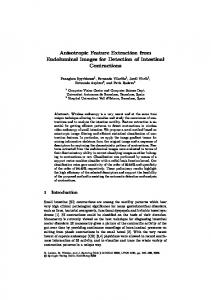
variability, Curran (1988). Durrieu et al. (2005) show that some textures have variograms that reflect certain periodicity in the image. Variograms often increase continuously with lag distance, however, the variogram is not restricted to such monotonic behavior and decreasing segments or periodicity can be observed. This variogram structures are identified as “hole effect” structures, and can offer valuable information which shouldn’t be discarded (Pyrcz et al., 2003). A periodic behavior indicates the existence of spatial structures in the images under study. At the same time this periodic characteristic of the variogram let us determine the window size to use. Different textures with their respective variogram curves can be seen in Figure 1:
1. INTRODUCTION Since its development in the mining industry geostatistics has been applied in different fields of study. However, in image analysis, and more specifically in texture analysis, the use of these techniques is relatively new. Different methods have been proposed to incorporate geostatistics to image analysis (see for example, Miranda et al. (1992, 1998), Chica-Olmo and Abarca-Hernandez (2000) or Maillard (2003)), with varying results. A well known tool used in geostatistics is the experimental semivariogram. From here on in this work we will be using the name variogram instead of experimental semivariogram. For continuous variables, such as reflectance in a given waveband, the variogram is defined as half the average squared difference between values separated by a given lag h, where h is a vector, in both distance and direction, Atkinson and Lewis (2000).
1 γ (h ) = 2N
∑ [Z (x ) − Z (x + h )] i
i
Fallow Fields
2420
19
1920
14
1420
Pine Trees 3167 2167
9
920
1167
4
420 1
2
3
4
5
6
7
8
9
10 11 12 13 14
1
15
2
3
Barren Soil
2
N
i =1
Orange Groves
4
5
6
7
8
9
10
11
12
13
167 1
2
3
4
5
Hortic. Crops
417
117 17 1
Function (1) relates semivariance to spatial separation and provides a concise and unbiased description of the scale and pattern of spatial
2
3
4 5
6
7
8
9 10 11 12 13 14 15 16 17
8
9
10 11 12 13 14 15
1160
320 270 220 170 120
317 217
7
Deg. Orange Groves
1360
(1)
6
960 760 560 360
1
2
3
4
5
6
7
1
2
3
4
5
6
7
8
9
10
11
12
13
Figure 1. Different textures with their respective variogram curves.
1
In this paper we determine that the range and the sill and other values of the variogram curve near the origin, provide useful information about the texture been studied. From these values, we determine different indices. In the cases where the variogram curve has a periodic behavior, more indices are extracted. Once these indices are obtained the most discriminant ones are chosen and a classification of the study area is made.
Subset 2 Figure 3. Subset 2: image of part of the city of Valencia
2. MATERIALS AND METHODS 2.1 Study area and data
2.2 Window size determination
The analysis was performed over two subsets of a QuickBird satellite image: Subset 1: From the panchromatic band of the image (0.61 m/pixel) (Figure 2). The area studied is located to the north of the province of Valencia, (Spain), and it is dominated by agricultural land with the primary production being oranges, as well as some cereal crops. There are also pine forests, mostly at the hill sides, with some outcrops of pine trees between the cultivated land. Six types of land cover classes were differentiated in order to test the usefulness of the method: forest, not cultivated land, cultivated with crops, cultivated with orange trees, cultivated with degraded orange trees, and young orange trees.
To incorporate this concept first we have to treat the digital number of each pixel as a variable, and as a realization of a random spatial process, and in that case a variogram can be calculated in each pixels neighborhood window (Chen and Gong, 2004), which size is determined as follows: The window size is an important parameter, due to the fact that has to be large enough to contain a representative part of the texture to which a single pixel belongs, but not as large as to include a part of an adjacent texture. In this study this issue is divided into two consecutive steps: 1) Omnidirectional Variogram: A fixed window size of 30 pixels is used. This size was considered large enough to account for all the variability present in the texture. An omnidirectional variogram is computed over this window. 2) Directional or omnidirectional variogram: We distinguish two cases according to the behaviour of the omnidirectional variogram computed in the first step, and the window size will be different depending on the result obtained. a) If the omnidirectional variogram presents periodicity, the size of the final window will be equal to the distance at which the second maximum value of the curve is reached. Over this window, eight directions are considered to compute the new variogram: 0°, 22.5°, 45°, 67.5°, 90°, 112.5°, 135° y 157.5°. Once these eight variograms are computed, the parameters are extracted from the variogram in the direction of maximum variability. b) If the omnidirectional variogram does not present periodicity, the window size will be the maximum possible, that is, 30 pixels. In this case, instead of a
Subset 1 Figure 2. Subset 1: image of cultivated land
Subset 2: It corresponds to the blue band of the same QuickBird image (2.4 m/pixel), resampled to 5 m/pixel, considered to be the most appropriate resolution for the average texture classes tested (Figure 3). This area contains a part of the city of Valencia. Four classes were defined: old urban areas, new building areas, facilities and industrial areas, parks and cultivated land.
2
directional variogram, the same omnidirectional variogram of the first step is used to extract the corresponding parameters.
Smp1 = hmax 2 − hmax1 Smp 5 =
2.3 Parameter extraction and selection
Gp 4 =
Variance γ (h1 )
h
b) First maximum parameters: Here we define the distance at which the expected range is reached, the mean of the values up to the expected range which we call the first maximum hmax1 , the variance of these values and different integrals up to that value. Fmp 1 = hmax 1 max1
1 Fmp 3 = max 1
max 1
)
The results of the classification of the urban area can be seen in Table 1. In this case, two analyses were made: (1) a classification with all the variogram derived indices in the first place, and (2) a classification adding the three visible spectral bands of the Quickbird image (resampled to 5 m.). Some control areas were determined in order to test the accuracy of the method. The parameters obtained from the variogram were compared with a well known texture analysis method, the cooccurrence matrix method, evaluating in each case the classification results. In the case of the cooccurrence matrix, eight parameters were used.
γ (h 2 ) γ (h1 )
1 max1
(
3. RESULTS
γ (h2 ) − γ (h1 )
Fmp 2 =
)
A low pass filter was applied over the original image and the result added to the set of the variogram parameters. The intention was to incorporate some information derived from the mean to the analysis, since the variogram provides only information regarding the spatial correlation of the data. A supervised classification of the two images described in paragraph 2.1, was made. The method of maximum likelihood was applied to the two subsets. This method assumes that the statistics for each class in each band are normally distributed and calculates the probability that a given pixel belongs to a specific class. Each pixel is assigned to the class that has the highest probability. Training samples of each representative area were defined. Edges were not included in the analysis although they have a mayor role in classification errors Ferro et al. (2002).
a) General parameters: In this category there is the ratio of the variogram value in the first two lags. We also consider ratio of the first variogram value and the variance of the data as an estimation of the sill. We also compute the slope at the origin, and different derivatives using the first three to four variogram values.
Gp 3 =
(
A more complete description of the parameters used is available in Durrieu et al. (2005).
The indices computed were based on mean values, variances and simple ratios between values at the first lag up to the first maximum value of the variogram, second derivatives of the values at the first lag and different integrals. If the result is a periodic variogram, a second set of parameters is computed. We consider that a variogram is periodic if it has a first maximum, a first minimum and a second maximum. Then, new parameters based on integrals and ratios between the first and the second maximum are computed. The parameters are divided into three categories:
Gp1 =
max 2 −1 h γ hmax1 + 2 ∑ γ (hi ) + γ hmax 2 2 i = max1 +1
The results in the three analysis carried out are very similar. The best result obtained was an overall accuracy of 76.4% with the co-occurrence matrix method. With all three methods the old and new city areas were difficult to discriminate.
∑ γ (hi ) i =1
∑ (γ (h ) − Fmp 2)
2
i
i =1
The results obtained in the classification of the agricultural area are shown in Table 2. In this case, the spectral bands were not included because it was considered that the information derived from the variogram was enough to give good results in a classification.
c) Second maximum parameters: This last set of parameters incorporate information extracted from the variogram of the values from the first maximum up to the second maximum.
3
derived from the variogram provide a better result in those classes with regularity and structural patterns, such as orange trees.
The results obtained comparing both methods are again very similar, although in this case the variogram method gives a better result, with an overall accuracy close to 84%. The parameters
Urban areas Semivariogram
Old City New City Industrial zone Parks and gardens Overall
Producers accuracy 83.8 70.4 57.9 81.5
Users accuracy 73.7 61.9 91.2 82.1 73.5
Semivariogram+spectral bands Producers Users accuracy accuracy 84.7 74.4 72.6 63.4 59.9 90.8 83.2 88.4 75.2
Co-occurrence Matrix Producers accuracy 88.9 71.3 64.3 81.4
Users accuracy 73.2 73.3 77.8 86.9 76.4
Table1. Classification results of urban areas comparing the semivariogram, semivariogram with spectral bands and co-occurrence matrix methods
Agricultural land
Crops Barren soil Orange groves Young orange groves Deg orange groves Pine trees Overall
Semivariogram Producers Users accuracy accuracy 100.0 93.3 94.2 100.0 90.1 87.1 69.7 71.2 62.6 64.4 100.0 100.0 83.9
Co-occurrenceMatrix Producers Users accuracy accuracy 97.5 98.5 99.3 98.8 90.0 90.8 57.2 73.1 77.1 52.7 99.0 100.0 82.9
Table 2. Classification results comparing the semivariogram and co-occurrence methods.
spatial structure as is the case of the orange groves from those textures that are more homogeneous as are barren soils. The intention to discriminate between different types of orange groves (mature, young and degraded) did not work as well as expected, especially between young and degraded orange groves, that were confused with each other.
4. CONCLUSIONS The use of an adaptative window size maximizes the within class variation reducing the between class variation and therefore reducing the so called “edge effect”. The method proposed takes into consideration two cases: a) variograms with periodic behavior where a direction is used. b) variograms without periodic behavior where an omnidirectional variogram is used. This distinction allowed us to better discriminate textures that present directionality or some kind of
The parameters proposed are valid, specially in the cases of textures with some structure. The parameters that better discriminate are those that include the first value of the variogram in any of its combinations.
4
Ferro, C.J.S., Warner, T.A., 2002. Scale and texture in digital image classification. Photogrammetric Engineering & Remote Sensing, 68 (1), 51-63.
5. REFERENCES Atkinson, P.M., Lewis, P. 2000. Geostatistical classification for remote sensing: an introduction. Computers & Geosciences, 26, 361-371.
Maillar, P., 2003. Comparing texture analysis methods through classification. Photogrammetric Engineering & Remote Sensing, 69 (4), 357-367.
Chen, Q., Gong, P. 2004. Automatic variogram parameter extraction for texture classification of the panchromatic IKONOS imagery. IEEE Transactions on Geostatistics and Remote Sensing, 42 (5), 1106-1115.
Miranda, F.P., MacDonald, J.A., Carr, J.R., 1992. Application of the semivariogram textural classifier (STC) for vegetation discrimination using SIR-B data of Borneo. International Journal of Remote Sensing, 13 (12), 23492354.
Chica-Olmo, M., Abarca-Hernández, F., 2000. Computing geostatistical image texture for remotely sensed data classification. Computers & Geosciences, 26, 373-383.
Miranda, F.P., Fonseca, L.E.N., Carr, J.R., 1998. Semivariogram textural classification of JERS-1 (Fuyo-1) SAR data obtained over a flooded area of the Amazon rainforest. International Journal of Remote Sensing, 19 (3), 549-556.
Curran, P.J., 1988. The semivariogram in remote sensing: an introduction. Remote Sensing of Environment, 24, 493-507. Durrieu, M., Ruiz, L.A., Balaguer, A., 2005. Analysis of geostatistical parameters for texture classification of satellite images. EARSeL Symposium - Global Developments in Environmental Earth Observation from Space (Ed. Andre Marcal), pp. 11-18. 6-8 June 2005, Porto, Portugal.
Pyrcz, M. J., Deutsch, C. V., 2003. The whole story on the hole effect. Searston, S. (ed) Geostatistical Association of Australasia, Newsletter 18, May 2003.
5