The C II Doppler shift precedes the O VI Doppler shift by 3Ñ
10 s. .... compensation for solar rotation. Thus ... The uncertainties in the measured Doppler shifts are.
THE ASTROPHYSICAL JOURNAL, 531 : 1150È1160, 2000 March 10 ( 2000. The American Astronomical Society. All rights reserved. Printed in U.S.A.
CHROMOSPHERIC AND TRANSITION REGION INTERNETWORK OSCILLATIONS : A SIGNATURE OF UPWARD-PROPAGATING WAVES ^. WIKSTÔL, V. H. HANSTEEN, AND M. CARLSSON Institute of Theoretical Astrophysics, University of Oslo, P.O. Box 1029, Blindern, 0315 Oslo, Norway
AND P. G. JUDGE High Altitude Observatory, National Center for Atmospheric Research,1 P.O. Box 3000, Boulder, CO 80307-3000 Received 1998 September 14 ; accepted 1999 October 27
ABSTRACT We analyze spectral time series obtained on 1997 April 25 with the SUMER instrument on SOHO. Line and continuum data near 1037 A were acquired at a cadence of 16 s. This spectral region was chosen because it contains strong emission lines of C II, formed in the upper chromosphere/lower transition region ; O VI, formed in the upper transition region ; and neighboring continuum emission formed in the middle chromosphere. The time series reveal oscillatory behavior. Subsonic (3È5 km s~1 amplitude) Doppler velocity oscillations in the C II and O VI lines, with periods between 120 and 200 s, are prominent. They are seen as large-scale coherent oscillations, typically of 3È7 Mm length scale, occasionally approaching 15 Mm, visible most clearly in internetwork regions. The Doppler velocity oscillations are related to oscillations seen in the continuum intensity, which precede upward velocity in C II by 40È60 s. The C II Doppler shift precedes the O VI Doppler shift by 3È10 s. Oscillations are also present in the line intensities, but the intensity amplitudes associated with the oscillations are small. The continuum intensity precedes the C II intensity by 30È50 s. Phase di†erence analysis shows that there is a preponderance of upward-propagating waves in the upper chromosphere that drive an oscillation in the transition region plasma, thus extending the evidence for upward-propagating waves from the photosphere up to the base of the corona. Subject headings : Sun : chromosphere È Sun : oscillations È Sun : transition region È waves 1.
INTRODUCTION
ed by a microchannel plate detector of size 1024 ] 360 pixels. The spatial resolution is 1@@ ] 2@@ (1A slit width, 1A sampling along the slit). The spectral resolution is about 40 mA in Ðrst order and 20 mA in second order. The data presented here were collected on 1997 April 25 and consist of a 3 hr time series, beginning at 02 : 05 UT, pointed at Sun center. In order to achieve high cadence but at the same time meet telemetry limitations, the number of wavelength pixels was limited to two 50 pixel wide (approximately 2 A ) windows, a ““ line ÏÏ window centered at j \ 1037.5 A and a ““ continuum ÏÏ window centered at j \ 1043 A . The line window contains the emission lines of C II and O VI. Immediately prior to these observations a full frame (1024 pixels) reference spectrum was obtained with an exposure time of 300 s. This allows an empirical wavelength calibration on the basis of the several chromospheric O I lines in the interval. Figure 1 shows the reference spectrum from 1030È1045 A averaged over a typical network and internetwork regions (the separation into ““ network ÏÏ and ““ internetwork ÏÏ is discussed below). The two 50 pixel wide time series windows are shaded gray in the Ðgure, and the lines we have identiÐed in the spectrum are indicated. Table 1 summarizes the essentials of the strongest spectral features. The region contains strong lines of O VI and C II, as well as chromospheric lines of O I that may be used for wavelength calibration. Note that both windows fall on the more sensitive (by a factor of 3.3) KBr coated part of the detector. This gives much better signal-to-noise ratio (S/N) than other data sets where the lines have been positioned on the bare part of the detector. The observed lines of O VI and C II have average count rates close to the maximum allowed count rate of 10 counts pixel~1 s~1.
To investigate the nature of and connection between the internetwork chromosphere and transition region, we have collected spectral time series data in the 1037 A region using the SUMER spectrograph (Wilhelm et al. 1995) on the SOHO spacecraft. The importance of this particular wavelength region is that it contains emission lines of C II formed in the upper chromosphere, a line of O VI formed in the upper transition region (temperature of formation about 300,000 K), and continuum emission formed in the middle chromosphere. These features can be observed simultaneously with SUMER while maintaining a high cadence. Here and in the following we use the terms ““ chromosphere ÏÏ and ““ transition region ÏÏ to denote temperature regimes rather than heights in a semiempirical static model. These regions are certainly dynamic and may be very fragmented and crinkled in loop structures. The observations can be used to relate time variations seen in the chromosphere to the transition region, in both network and internetwork. We focus mainly on internetwork regions, but similarities and di†erences between network and internetwork are also discussed. Our emphasis is on deriving empirical properties of the time series data, leaving numerical simulations for future work. 2.
OBSERVATIONS AND DATA REDUCTION
The SUMER instrument images areas of the Sun with a small SiC telescope and passes the light to a normal incidence stigmatic spectrograph. The di†racted light is record1 The National Center for Atmospheric Research is sponsored by the National Science Foundation.
1150
INTERNETWORK OSCILLATIONS
FIG. 1.ÈTime-averaged reference spectrum for a typical network region (solid line ; averaged over spatial positions 10È44 along the slit) and a typical internetwork region (dashed line ; averaged over positions 45È69). The gray areas mark the two 50 pixel windows read down at each time step.
The exposure time for the time series is 12 s, but because of operational overhead the e†ective cadence was limited to 15.8 s. We used a 1@@ ] 120@@ slit, Ðxed at Sun center without compensation for solar rotation. Thus, new areas of the Sun drifted into the slit as the Sun rotated beneath, on a timescale of 383 s. An area of approximately 30@@ ] 120@@ is mapped during the time series. The data reduction procedure involved Ñat Ðelding, geometric correction, and wavelength and radiometric calibration. These steps were performed as described by Carlsson, Judge, & Wilhelm (1997), Judge, Carlsson, & Wilhelm (1997), and Hansteen et al. (2000). SUMER ÑatÐeld exposures were on average taken only once per month in 1997. The Ñat-Ðeld exposure used here was taken the day before the observations, leading to much cleaner Ñat Ðelding than normal with SUMER data. SUMER lacks an onboard calibration lamp, so the wavelength scale must be determined relative to reference lines in the solar spectrum itself, typically chromospheric lines from neutrals or singly ionized atoms. Unfortunately, the apparent separation of the di†erent reference lines in the data are inconsistent with laboratory wavelengths, meaning that somewhat di†erent wavelength scales can result depending TABLE 1 IDENTIFICATION OF SPECTRAL LINES : THE STRONGEST SPECTRAL FEATURES IDENTIFIED BETWEEN 1030È1045 A j (A )
Ion
T (K)
1031.912 . . . . . . 1036.337 . . . . . . 1037.018 . . . . . . 1037.613 . . . . . . 1039.230 . . . . . . 1040.943 . . . . . . 1041.688 . . . . . .
O VI C II C II O VI OI OI OI
300,000 20,000 20,000 300,000 10,000 10,000 10,000
NOTE.ÈThe temperatures in the right column indicate the approximate temperatures of formation of the lines in equilibrium.
1151
on which lines are included in the calibration. The same wavelength region has been studied with SUMER by Warren, Mariska, & Wilhelm (1997). They found that the Doppler shifts of the O VI 1031.912 and 1037.613 A lines were not self-consistent. The origin of these discrepancies is unclear. Inspection of the data used by T. Moran (1997, private communication) to determine the geometric correction (dewarping using spline interpolation) revealed that, for detector B, the errors in the spline interpolation are anomalously large between wavelength pixels 250 and 320. The C II and O VI data were acquired on this part of detector B (Fig. 1). We therefore adopt a wavelength calibration using the O I lines closest to the O VI line on the longward side, and the C II 1037.018 A line itself. All wavelength measurements are relative to the O I and C II lines. We emphasize that this deters us from making a good absolute wavelength calibration but does not a†ect the reported relative Doppler shifts. The uncertainties in the measured Doppler shifts are mainly due to counting statistics. Typical count rates in network regions imply Doppler velocity errors of about 2 km s~1 for C II j1037 and 1 km s~1 for O VI j1037. The corresponding values for the fainter internetwork regions are 3.5 and 1.5 km s~1. The radiometric calibration was taken from Wilhelm et al. (1997). 3.
RESULTS
3.1. Underlying Photospheric Magnetic Structure No supporting data were acquired speciÐcally in support of the SUMER observations, so we are unable to specify the exact state of the magnetic Ðeld emerging from beneath the photosphere during the SUMER observations. Nevertheless, the MDI instrument on SOHO was running in a mode where full disk (2A pixel~1) magnetogram data were obtained every 96 minutes. Comparisons of these data with the SUMER data indicate that the SUMER pointing (the center of the slit) was close to (]10A, ]20A). The MDI data reveal that the region scanned (by solar rotation) under the SUMER slit was in a typical quiet region, mostly unipolar, with a moderately intense network element near the north end of the SUMER slit. On the basis of this crude (by-eye) coalignment, we assign the bright network element in the MDI data to pixels 10È44 in the SUMER time series (pixel 0 is the northernmost pixel in SUMER). The region between SUMER spatial pixels 70È90 can also be classiÐed as network, with pixels 45È69 as internetwork. The exact limits of the network/internetwork regions are not clearly deÐned. The MDI data also show only small time variation changes in the photospheric network Ðelds during the time series. Furthermore, a more sensitive high-resolution (0A. 6 pixel~1) magnetogram image, which includes the region spanned by the SUMER slit, was obtained later at 09 : 11 UT. Based on these data, we conclude that the SUMER time series data set corresponds to typical quiet-Sun conditions. The unsigned magnetic Ñux for all pixels within 10A of the position of the area scanned by solar rotation under the projected SUMER slit (i.e., a 40@@ ] 140@@ area), above the 20 G pixel~1 sensitivity limit, was ^4 Mx cm~2. 3.2. Intensity and Doppler Shift Maps Figure 2 illustrates continuum intensities as a function of position along the slit (abscissa) and time (ordinate). Figure
1152
WIKST^L ET AL.
FIG. 2.Èj1043 continuum intensity in radiation temperature (K) as a function of position along the slit and time. Notice the distinct oscillations in the internetwork areas between spatial bins 45 and 70, and higher than 85.
3 shows maps of intensity and Doppler shift for the C II and O VI lines. The background continuum intensities, estimated from the 1043 A window, were subtracted from the line proÐles prior to measuring them. The Ðgure shows that the continuum intensity variations are small in the network, and no obvious patterns are seen. In contrast, the internetwork regions display distinct oscillatory behavior of the continuum. These oscillations are typically coherent
over a few pixels, sometimes up to 10A, and are apparent most of the time in all internetwork areas. The oscillation periods are typically 100È200 s. The network/internetwork boundaries in the SUMER data are indicated with dashed lines in Figure 3. The region above spatial pixel B90 contains both bright and darker emission, but at least for the latter half of the time series it seems fair to call it internetwork. Table 2 contains a
FIG. 3.ÈL eft : Intensity for (upper ) C II and (lower) O VI. Right : Doppler velocity for same. Intensities are W m~2 sr~1 according to inset gray scale. Negative Doppler shifts (blueshifts) are coded lighter shades, according to the scale. Dashed lines in the left panels indicate the regions chosen to represent the network and the internetwork areas. The internetwork Doppler shift shows a clear oscillatory behavior.
1154
WIKST^L ET AL. TABLE 2 SUMMARY OF INTENSITY AND DOPPLER SHIFT CHARACTERISTICS INTENSITYa Networkb
DOPPLER SHIFT (km s~1)
Internetworkc
Network
Internetwork
FEATURE
Mean
rms
Mean
rms
Mean
rms
Mean
rms
Continuum . . . . . . C II . . . . . . . . . . . . . . . O VI . . . . . . . . . . . . .
5331 0.06 0.16
79 0.028 0.09
5218 0.016 0.06
71 0.007 0.026
... 1 7
... 3.5 5.8
... [1 5
... 4.6 6.5
a Intensities are in radiation temperature (K) for the continuum and in W m~2 sr~1 for the lines. b Averaged over spatial positions 10È44. c Averaged over spatial positions 45È69.
summary of the basic characteristics of continuum and line intensities and line Doppler shifts for these internetwork and network regions. Comparison of Figures 2 and 3 reveals that the network/ internetwork patterns seen in the continuum intensity are also present in the line intensities. On average the O VI line is a factor of 2.8 brighter than the C II line in the network, although the O VI and C II line network intensity variations are similar. The network intensity is continually changing on timescales shorter than 383 s in both lines. Typical timescales are 100È300 s, but examples of more rapid variations can be found occasionally in both lines. Brightenings by a factor of 1.5È2 are frequently seen on these timescales, occurring more often in the hotter (O VI) line. The typical spatial scale of a brightening event is 3AÈ10A. On smaller scales there are both temporal and spatial di†erences between the lines. In most cases a brightening of one of the lines can also be found in the other, but the relative strengths of the events are generally di†erent, they are often displaced by 1AÈ2A, and they frequently occur at slightly di†erent times. The rms values of intensity variations in Table 2 show that the amplitudes of intensity variations are slightly larger in the hotter line. Although the internetwork region appears very dark in the line intensities in Figure 3, it is important to stress that we do see emission in both lines everywhere at all times. The intensity contrast between the two lines is larger in internetwork than in network regions (the O VI line being about 4 times brighter than the C II line). The internetwork intensity varies almost everywhere at all times, with rms variations that are slightly smaller than those found in the network. As shown in Table 2, the O VI line is redshifted in both network and internetwork regions, but the net shift is slightly larger in the former. The C II line is on average slightly more redshifted in the network than in the internetwork. The rms values represent the magnitudes of typical Doppler shift variations. These are larger in the hotter line, and in both lines the rms values are higher in internetwork than in network regions. Now, consider the Doppler shifts in the internetwork regions of Figure 3. A distinct oscillatory behavior is found in both O VI and C II. These oscillations are often spatially coherent over 5AÈ10A, sometimes even more, and have periods of 100È200 s, peaking around 170È200 s. The amplitudes typically are ^4È5 km s~1 in C II and ^3È4 km s~1 in O VI. For reference, the sound speeds are roughly 15 and 85 km s~1, respectively. The spatial extents of the oscillating regions are slightly larger in O VI, occasionally much larger
(e.g., spatial pixels 50È70, and times greater than 8000 s in Fig. 3). Details of these oscillations are shown in Figure 4, which displays (upper left panel) continuum intensity, (lower left panel) C II intensity, (upper right panel) C II Doppler velocity, and (lower right panel) O VI Doppler velocity in the internetwork region between spatial positions 45È65 for a selected time span of about 3000 s. Distinct continuum oscillations are ubiquitous. The typical width of an oscillating region is 5AÈ10A (e.g., pixels 53È58, t ^ 2800 s), but sometimes regions as large as an entire supergranular cell (^20A) seem to oscillate coherently. The continuum correction is constant over the extent of the line proÐle and thus would be very unlikely to a†ect the line shift. Oscillations in the line intensity of C II are much smaller in amplitude than in the continuum. However, closer inspection reveals that oscillations can also be seen in the line intensity. For example, the bright event in continuum intensity at t ^ 2800 s is also found in the C II intensity slightly later in time, with less strength. Oscillations are present in the Doppler shift maps of both lines. The continuum feature near 2800 s, the brightest event in the Ðgure, coincides with a blueshift of 4 km s~1 in C II preceded by a redshift of 4 km s~1 but is almost invisible in the O VI Doppler shift. In general continuum brightenings often precede blueshifts in the lines by 30È60 s. The spatial scales are also similar in the intensity and Doppler shift oscillations. When broad oscillatory regions appear in continuum intensity, the oscillating regions are also broader in line Doppler shift (e.g., compare continuum intensity with O VI Doppler shift from 3000È3500 s). We will return to the issue of possible phase relations in ° 3.4. 3.3. Power Spectra The left panel of Figure 5 displays the j1043 continuum intensity as a function of time at typical positions in the network (dashed line) and internetwork (solid line). The intensity Ñuctuates continuously at both slit positions, with similar amplitudes. While no particular periodicity is evident in the network, the internetwork intensity clearly has periodic components. Power spectra of the continuum intensity in both network and internetwork regions are shown in the right panel of Figure 5. The time signals were treated using the ““ Hann ÏÏ windowing function before Fourier transformations were applied. The right panel shows the average power in the network area between spatial positions 10 and 44 (dashed line) and in the internetwork area between spatial positions 45 and 69 (solid line). The power was calculated by averaging the intensity
FIG. 4.ÈContinuum intensity in (upper left) radiation temperature, (lower left) C II intensity, (upper right) C II Doppler shift, and (lower right) O VI Doppler shift in a selected time slice of a typical internetwork area.
1156
WIKST^L ET AL.
FIG. 5.ÈL eft : Continuum intensity as a function of time at a network slit position (x \ 40 ; dashed line) and an internetwork position (x \ 53 ; solid line). Right : Power spectra calculated from such time series averaged over a typical network region (spatial bins 10È44 ; dashed line) and an internetwork region (bins 45È69 ; solid line. The 1 and 2 p noise levels in the internetwork (dotted line) are shown. The Nyquist frequency is 31.5 mHz.
power calculated at each individual spatial position. The dotted lines indicate the 1 and 2 p noise levels in the power spectra. The noise was estimated by computing the power contained in random, artiÐcial data with the same average intensity as the real data at each spatial position. Displayed in the Ðgure is the average of the estimated noise found at high frequencies. The noise level plotted is representative of typical internetwork regions ; noise in network regions is correspondingly smaller.2 The most striking feature is the dramatic increase in the internetwork power from 3 to 8 mHz (periods from 330 to 125 s). The maximum power is around 5 mHz (200 s). The network shows high power at low frequencies and a peak at 3È4 mHz. Thus, it seems evident that some wave phenomenon with periods peaking at 200 s dominates the dynamics of the chromosphere at the height of the 1043 A continuum, which forms close to 1.1 Mm (above q \ 1) in model C of Vernazza, Avrett, & Loeser (1981). 5000 Figure 6 shows power spectra of the (upper panels) intensity and (lower panels) Doppler shift for the C II and O VI lines. The power is averaged over the same network and internetwork areas as in Figure 5. First, consider the power spectra of C II j1037. The intensity power is similar in the two regions, and they both show exponential decay with increasing frequency. The exceptions are three peaks in the internetwork power seen at 2È3, 4, and 5 mHz. The Doppler shift power spectra show considerably more power at higher frequencies. The internetwork power spectrum displays a dramatic increase in power around 3.3È8 mHz (periods from 300 to 125 s), again peaking near 5 mHz. In the network the picture is strikingly di†erent, with only a small increase in power at 3È4 and at 5.5 mHz. The general behavior is seen also for O VI, where no strong features are found in the intensity signal, although 2 One should keep in mind that as a result of solar rotation the power may increase at frequencies below 2.6 mHz. There is also an instrumental drift in the Doppler shift with a period of a few hours that will contribute to the power at the lowest frequencies. These considerations limit the validity of noise estimates to frequencies above 2.6 mHz.
the internetwork power between 2 and 5 mHz is slightly higher than a completely random signal. The internetwork Doppler shift of O VI shows behavior similar to that of C II, with a dramatic increase in power between 3 and 7 mHz : the largest peak is located, once again, at 5 mHz (200 s). Thus, oscillations with periods in the range of 125È300 s are a dominant feature in the continuum intensities and in the Doppler shifts, at the resolvable scales. In line intensities, the oscillations are much less pronounced. 3.4. Phase Shifts Basic considerations of the physics of wave propagation in the nearly isothermal chromosphere, with the steep temperature gradient transition region as its upper boundary, lead us to expect phase delays between the continuum and the C II and O VI oscillations. On the basis of linear theory (e.g., Mihalas & Mihalas 1984), waves excited in lower atmospheric layers should yield a continuum intensity signal that precedes the transition region intensity and Doppler shift signals by amounts that depend on the frequency of the oscillations and on the fraction of the wave energy Ñux reÑected on the transition region. If the waves are totally reÑected, the velocity (Doppler shift) and density (intensity) signal will be 90¡ out of phase for each of the ions, and the various intensity signals will either be in phase or 180¡ out of phase. With partial reÑection the Doppler shift and intensity signals will have phase di†erences that depend on their locations and on the relative amount of reÑection. In order to explore the possible phase relations between the oscillations seen in the intensities and Doppler shifts of the two lines and in the continuum intensity, we selected a time period in the internetwork region that reveals in Figure 4 particularly strong oscillations. Figure 7 shows continuum intensity (solid line), C II Doppler velocity (dotted line), and O VI Doppler velocity (dashed line) as a function of time for a period of about 1200 s, averaged over spatial pixels 51È53. Upward velocity is positive. It is obvious that the oscillations seen in the continuum intensity are connected to the Doppler shift oscillations in the lines formed higher up in the chromosphere and the
FIG. 6.ÈT op : Power spectra of C II and O VI intensities and averaged over the same regions as in Fig. 5. Bottom : Doppler shifts averaged over same regions. The noise levels (dotted lines) are estimated from internetwork areas. In the network, the noise level is roughly a factor of 2 lower. Notice the peaks in internetwork Doppler shift in both lines.
1158
WIKST^L ET AL.
FIG. 7.ÈContinuum intensity (solid line), C II Doppler shift (dotted line), and O VI Doppler shift (dashed line) in a selected time interval. All quantities have been averaged over spatial pixels 51È53, typical internetwork positions, and normalized so that each curve has the same range in the Ðgure [corresponding to (5165, 5357) K in continuum intensity radiation temperature, ([5.0, 6.7) km s~1 in C II Doppler shift, and ([3.2, 6.1) km s~1 in O VI Doppler shift]. Negative Doppler shifts (blueshifts) are upward in the Ðgure.
transition region. These data are consistent with the behavior expected from linear theory for predominantly upwardpropagating waves, since the continuum intensity oscillations (formed near 1 Mm) appear to precede the Doppler shift oscillations (assumed to be formed nearer to 2 Mm). The Doppler shift signals seem to be nearly in phase but with the C II Doppler shift slightly ahead of O VI. Time delays of 50 s between continuum intensity and C II Doppler shift and 4 s between C II and O VI Doppler shifts were determined from a simple cross-correlation between the intensity and Doppler shift images 3 spatial pixels wide. This evidence suggests that the transition region oscillations are a manifestation of upward-propagating waves. To investigate this further and to exclude the possibility that the oscillatory signal is due to a purely standing wave, we calculate the time delays for the intensities and Doppler shifts and their uncertainties at all spatial positions. Uncertainties in the time delays are estimated as follows. At each spatial position we divide the Doppler shift time series into three subsets and calculate the time delay using the crosscorrelation technique at each position along the slit for the three temporal subsets. This procedure is repeated 100 times, and each time artiÐcial noise is added to the Doppler shift and intensity signals and new phase shifts are calculated. The noise added is randomly selected from Gaussian distributions whose widths were set to the estimated errors in the Doppler shift scales (3.5 and 1.5 km s~1 for C II and O VI, respectively, in the internetwork ; see ° 2). We thus obtain 100 realizations at each spatial position and temporal subset, and the errors were estimated to the standard deviations.
Figure 8 depicts the time delays as a function of the position along the slit between (top panel) C II and O VI Doppler shifts, (second panel) C II Doppler shift and continuum intensity, (third panel) C II and continuum intensities, and (bottom panel) C II Doppler shift and intensity. One sees a clear correlation between the phase shifts and the brightness of the regions. In internetwork regions (spatial positions 45È69 and 90È110) the C II Doppler shift leads the O VI Doppler shift by 3È10 s. In several of the brighter regions the data indicate that the O VI Doppler shift might precede the C II Doppler shift by 1È2 s. This suggests that di†erent mechanisms dominate the transition region dynamics in network and internetwork regions. The continuum intensity leads the C II Doppler shift by about 50 s. This is consistent with an upward-propagating wave or with the 90¡ phase shift (for a 200 s period) expected between density and velocity in a standing wave. We favor the Ðrst interpretation for a number of reasons. First, the third panel shows a clear time delay between the continuum intensity and the C II intensity. This result is consistent with a wave Ðeld dominated by upward-propagating waves but not standing waves. Second, a standing wave extending all the way from the formation height of the continuum to the transition region would require not only large reÑection from the transition region but also very little radiative damping of the wave. Third, the bottom panel shows only a small phase di†erence between the Doppler shift and intensity in the C II line. In a standing wave this phase di†erence would be expected to be 90¡ (50 s). A wave Ðeld dominated by propagating waves but with some reÑection is consistent with the observed time delay of 10È20 s between C II intensity and Doppler shift. Last, we can analyze the phase delays as a function of frequency from the Fourier analysis using previously established techniques applied to the photosphere and lower chromosphere (Lites, Rutten, & Kalkofen 1993). Figure 9 shows the phase delay between the continuum intensity and the C II Doppler shift, as a function of frequency, for all points classiÐed previously as internetwork, for the duration of the time series. The data are consistent with increasing phase with increasing frequency between 3 and 7 mHz, a clear signature of upward propagation (e.g., Lites et al. 1993). The lower panel shows the phase coherence, showing that for a signiÐcant fraction of the entire time series, the 3È7 mHz oscillations are coherent, indicating that a large fraction of the oscillations are indeed upward propagating and are not just manifestations of noise (which would yield random phases with lower coherence levels seen at higher frequencies). Thus, we believe that these data extend the evidence previously found for upward-propagating waves from the photosphere up to D1 Mm (Lites et al. 1993) to the 2 Mm level at the base of the corona. 4.
CONCLUSIONS
This work has revealed the presence of small-amplitude (subsonic) Doppler shift oscillations, with periods of 120È200 s, in plasma canonically at lower and upper transition region temperatures. The intensity variations associated with the Doppler shift oscillations are small but possibly consistent with acoustic waves with the measured velocity amplitudes. The Doppler shift oscillations are demonstrably connected to continuum intensity oscillations formed in the underlying chromosphere. They occur most often between regions of strong network emission but can
FIG. 8.ÈPhase shift (diamonds) as a function of position between (top panel) C II and O VI Doppler shifts, (second panel) C II Doppler shift and continuum intensity, (third panel) C II and continuum intensities, and (bottom panel) C II Doppler shift and intensity. In each case a positive time delay is consistent with upward propagation, i.e., in the top panel a positive phase indicates that C II Doppler shift precedes O VI Doppler shift. For reference we also show in each panel the time-averaged intensity in the O VI line (solid lines). Estimated errors in the time delays are indicated at (upper panel) spatial positions 55 and 85 and (remaining panels) bin 55. There is a clear tendency for positive phase shifts in internetwork regions.
1160
WIKST^L ET AL.
FIG. 9.ÈPhase di†erence (upper panel) and phase coherence (lower panel) for the Fourier phase spectra of the continuum intensity and C II Doppler shift. A positive phase di†erence implies that the continuum intensity precedes the C II Doppler shift. The points show a scatter plot of (upper panel) the phase di†erences and of (lower panel) the coherences ; the symbols in the upper panel show mean and rms variations, and the solid line in the lower panel shows the mean behavior of the phase coherence. The coherence peaks close to 5 mHz and is signiÐcantly above the noise level between 3 and 7 mHz, a region showing a trend of increasing phase with frequency. As stressed in the text, this is a clear signature of an upward-propagating wave phenomenon.
be seen at times in the network itself. These oscillations are found ubiquitously in internetwork areas and are coherent over typically 5AÈ10A scales, and the coherent regions appear to be broader in the upper transition region than at
the top of the chromosphere. These scales are much larger than implied by many spectroscopic studies, which deduce that the transition region is extremely Ðnely structured (e.g., see the discussion by Mariska 1992). This apparent contradiction might not be a contradiction at all since a Ðnely structured medium can respond coherently to a large-scale acoustic disturbance. These data demonstrate that a relatively coherent wave phenomenon may be present all the way from the middle chromosphere (1 Mm) up through the upper transition region (2 Mm and higher). Based on phase relations between the continuum intensity and the line intensity and Doppler shift signals, we argue that the oscillations are a manifestation of waves propagating upward in the atmosphere. The time delay between the C II Doppler shift relative to the O VI line is also consistent with this picture. The opposite phase relation found between the Doppler shifts in the network indicates that the waves may propagate downward in these regions, but more work is needed to settle this issue since the phase shifts measured are small and the data are noisy.
This work was supported by grant 121076/420 from the Norwegian Research Council.
REFERENCES Carlsson, M., Judge, P. G., & Wilhelm, K. 1997, ApJ, 486, L63 Mihalas, D., & Mihalas, B. W. 1984, Foundations of Radiation HydrodyHansteen, V. H., Betta, R., Carlsson, M., & Wilhelm, K. 2000, ApJ, subnamics (New York : Oxford Univ. Press) mitted Vernazza, J. E., Avrett, E. H., & Loeser, R. 1981, ApJS, 45, 635 Judge, P. G., Carlsson, M., & Wilhelm, K. 1997, ApJ, 490, L195 Warren, H. P., Mariska, J. T., & Wilhelm, K. 1997, ApJ, 490, L187 Lites, B. W., Rutten, R. J., & Kalkofen, W. 1993, ApJ, 414, 345 Wilhelm, K., et al. 1995, Sol. Phys., 162, 189 Mariska, J. T. 1992, The Solar Transition Region (Cambridge : Cambridge Wilhelm, K., Lemaire, P., Feldman, U., Hollandt, J., Schuhle, U. H., & Univ. Press) Curdt, W. 1997, Appl. Opt., 36, 6416