XV International Symposium on High Voltage Engineering th. University of Ljubljana, Elektroinštitut Milan Vidmar, Ljubljana, Slovenia, August 27-31, 2007.
XVth International Symposium on High Voltage Engineering University of Ljubljana, Elektroinštitut Milan Vidmar, Ljubljana, Slovenia, August 27-31, 2007
T7-547.pdf
New Procedures for Partial Discharge Localization in Gas-Insulated Switchgears in Frequency and Time Domain Stefan M. Hoek 1* , Uwe Riechert 2, Thomas Strehl 3, Kurt Feser 1 and Stefan Tenbohlen 1 1 University of Stuttgart, IEH, Pfaffenwaldring 47, 70569 Stuttgart, Germany 2 ABB Switzerland Ltd - Gas Insulated Switch Systems, Zürich, Switzerland 3 LEMKE DIAGNOSTICS GmbH in Volkersdorf, Dresden, Germany
Abstract: This paper introduces to new methods providing a cost-efficient localization of partial discharges (PD) in gas-insulated switchgears (GIS). A new analogue signal-processing unit minimises necessary equipment for a time-of-flight measurement (time domain) by means of time-to-digital (TDC) converters. The analogue signal processing unit recognizes the beginning of the UHF-signal and acquires start and stop commands for the TDC. The TDC measures the time difference (Δt), which is necessary to localize the PD. Another method uses the interference phenomenon of two superimposed sensor signals in the frequency domain. The signal interference is generated by the time delay (Δt) between the signals. Two similar sensor signals are required to receive acceptable results for the measurement procedure. Considering the dispersion effects of higher modes in GIS only a certain frequency range is useful for the measurement. At various setups the interferences were measured. Both methods are able to evaluate the time delay between the sensor signals and to localize PD in GIS in a cost-effective way.
sectionizing, electrical time-of-flight measurements, acoustic measurement and a combination of them . Other newly investigated methods are the interference measurement in the frequency domain or the measurement with a simple setup in time domain. The advantage of these methods is less equipment effort compared to nowadays used localization methods in time domain. 2.1 Localization in Time Domain Very fast electric pulses with rise times below 1 ns, emitted by a PD source, propagate in all directions along the GIS duct. A simple and obvious way of locating is a measurement with the time-of-flight method. Here the time difference between the wave fronts arriving at two UHF-PD-sensors indicate the location of the PD source. The time difference (∆t) is usually in tens of 1 ns, so that a fast digital acquisition has to be applied for measurements [3].
1 INTRODUCTION To optimise processes in utilities a condition based maintenance strategy is essential. The liberalization of the energy market forces utilities to reduce costs. Considering the maintenance strategy of GIS, a sensitive PD detection is important. To identify the type of the PD, various proven methods are possible, like the analyses of the phased resolved partial discharge (PRPD) diagram or other techniques. To assess the risk of a defect the location is additionally important. Thus, a sensitive PD detection with estimation of the nature of the defect and a fast and exact localization is advantageous. Hence the demand for reliable and economic measurement tools to locate PD-sources increases.
2 PD LOCALIZATION IN GIS Several methods can be used based on different physical phenomena. Methods based on a time delay evaluation between different propagating modes [1] and directional co uplers [2], have shown to be unpractical [3]. The most practical methods are based on
Fig. 1: Longitudinal section of a GIS
The distance X1 can be calculated with the equation (1) in case the time difference (∆t) is known. X represents the distance between the sensors and c0 is the propagation speed of the wave in the GIS (c0 = 0.3 m/ns) [3]. The constant propagation speed of the wave is an important pre-condition for localization. X1 =
X − ( X 2 − X 1 ) X − c 0 ⋅ ∆t = 2 2
(1)
The time difference ∆t is determined by the time delay between two signals. The identification of the signal beginning with an oscilloscope is not simple. Low signals and limited slopes are reasons for scattered results.
1
It is possible to replace the necessary fast digital acquisition equipment by means of fast time-to-digital converters (TDC) (resolution e.g. < 100 ps). The TDC measures the time difference (∆t) between a digital start and stop command. An electronic circuit was developed including a TDC and an analogue signal processing. The analogue signal processing converts the UHF-signal into digital commands. The first digital command of the signal-processing unit starts the time measurement. The digital command of the other signal processing stops the counter. The analogue signal-processing unit determines the starting point of the UHF-Signal to generate the digital command for the TDC. A well-proven method is to investigate the power of the signal. A noticeable rising of the signal power is a good indicator for PD [4]. By using the power of the signal its possible to detect UHFPD-signals, which are close to the noise level. The output signal, which depends on the input power, is generated by a fast commercial power detector (PwD) with an amplifier (Fig 2). The noise of the UHF-sensor signal is nearly constant and leads to an offset of the output signal of the PwD. In our case a negative slope indicates an increase of input power.
12
analogue signal processing unit
start
time-to-digitalconverter
x10
3-
A B
10 8 6
V
TDC
4 2 0 2 4 -
analogue signal processing unit
stop
0
S1
1
2
s
3
4
5
6 -7 x10
S2
Microcontoller Sensor 1
Sensor 2
el. PD -Impuls
X X1
X2
Fig. 3: Measurement system
2.2.1 Requirements The asymmetry of the signal strength of the UHF input channels have under certain conditions an influence on accuracy of the measurement (Fig 4). 5 ns 0
time delay t
2.2 Localization with a Simple Setup in Time Domain
-5 -10
< 50pC
-15
< 30pC < 15pC
-20 0dB
3dB
6dB
9dB
20dB
asymmetic attenuation
Fig. 4: Time delay caused by asymmetric signal power
An important requirement is the knowledge about the GIS. For example it is essential to know the position of disconnectors, because a discontinuity of the conductor leads to an additional attenuation and time delay.
Fig. 2: In- and output signal of the PwD
A comparator converts the analogue power signal of the PwD using a trigger level into a digital command for the time measurement. The trigger level can be a fixed value or it is generated by the analogue power signal itself. A trigger level near the noise level gives the best results. By using fast electronically devices, it’s possible to create an output signal, which is qualified to trigger the TDC. A microcontroller is necessary to control the TDC, transmit the results and process the data. Fig 3 shows the complete measurement system.
2.2.2 Measurement The analogue signal-processing unit was tested at a GIS in the laboratory (Fig 9). The start point of the signal was evaluated with a PwD and a comparator with a fixed trigger level. The PD-source was a pulse generator with an antenna, which was moved through the GIS between two sensors. By using this method, the accuracy of the time difference was better than 2 ns (Fig 5). The sensitivity of the system is sufficient to localize PD with a charge below 5 pC. The sensitivity depends on the type of GIS, PD sensors and distance between sensors. Further investigations on-site have to prove the sensitivity under real conditions.
2
14
time delay Δt
H (ω ) ω ⋅ ∆t = K t (ω ) = cos F (ω ) + G (ω ) 2
theoretical
ns 12
fixed tigger level
10
(6)
This cosine function has equidistant minima (see Fig 6), which can be interpreted as interference phenomena [5].
8 6 4
0
2 -10
360
310
260
210
160
110
60 cm
[dB]
0 10
distance Δs
-30
Fig. 5.: Time delay measurement in the laboratories GIS
1200
[(
)] = FFT [ f (t )] ⋅ e
(2)
2.3.1 Measurement Procedure To visualise the interference phenomena it is insufficient to make only one measurement. There are three power spectrums needed, which are compared in a characteristic way. The power spectrum is the absolute value of the complex FFT. The three power spectrums are obtained from Sensor 1 in equation (3), Sensor 2 in equation (4) and the added signal of Sensor 1 and 2 in equation (5) with a conventional spectrum analyser. The last signal is obtained with a RF power splitter, with no further reflections or other disturbing influences (Fig. 10).
F (ω ) = FFT [ f (t )] G (ω ) = FFT [g (t ) ] H (ω ) = FFT [g (t ) + f ( t − ∆ t ) ]
1300 1350 Frequency [MHz]
1400
(3) (4) (5)
The distance between the minima is defined as interference frequency ∆f. The ∆t is calculable by (7).
1 (7) ∆f At least two measurements with different cable length are necessary for a localization, because the result time delay |Δt| is an unsigned value (Fig. 10). ∆t =
2.3.2 Requirements Two related signals are required to obtain useful results from equation (6). Current studies show that a magnitude difference is not critical if the nature of both signals is similar. For different magnitudes, the combined function (6) changes to the absolute value of a cosine function with decreased magnitude and an offset. To keep the characteristics of both signals similar the effect of dispersion should be kept as small as possible. [5] 1800 1600 Critical frequency (MHz)
Another method to localize PD in GIS is to use the frequency domain. The interference phenomena of two sensor signals, which are added, should give information about the time delay (Δt) between the signals. A measurement procedure with a spectrum analyser instead of a cost-intensive fast digital oscilloscope will be more economical. The idea is based on the time-shift property of a Fourier Transformation of the received signals. − jω∆ t
1250
Fig. 6.: Resulting cosine function from (6) for a ∆t = 40 ns
2.3 Localization in Frequency Domain with Interference Measurement
FFT f t − ∆ t
ω ⋅ ∆t cos 2
-20
550 kV
1400
362 kV
1200
300 kV
1564 1404 1133
1000 991
800
717
600 521
400
377
200
1651
1196
1016
721
805
851
508
267
0
These three resulting signals are combined in (6). The time difference (∆t) is definable with the resulting cosine function in case of f(t) = g(t).
TEM
TE11
TE21
TE31
TM02
TE02 / TM11
Wave modes
Fig. 7.: Critical frequencies (fc) within a GIS for 300 kV, 362 kV and 550 kV
Three different types of wave modes, which propagate in GIS, are distinguished. The TMmn-mode
3
(Hz = 0), the TEmn-mode (E z = 0) and the TEM-mode (Hz = 0, E z = 0) (m and n mark the different types of wave modes). Every wave mode, except the TEMmode, has its own critical frequency (f c ). Higher modes are able to propagate at frequencies above their own critical frequency (f c ). TEM-modes have no critical frequency and will propagate starting from 0 Hz. The critical frequencies depends on the geometry of the GIS. With an increasing cross section of the GIS, the critical frequency is decreasing. In figure 7 the critical frequencies of the first wave modes are shown for three different types of GIS [6]. The group velocity (v g) of the TE- / TM-wave modes is frequency dependent which is a precondition for dispersion. The spe ed of higher wave modes can be calculated according to the following equation.
fc (8) f Below the lowest critical frequency of all modes (in GIS the f c of TE 11), only TEM-modes are able to propagate [7]. In this frequency range less dispersion effects exists and the interferences can be recognized. To measure in the frequency range below the first critical frequency, a low pass filter is applied, because the signal energy in the higher modes is much higher than in the TEM-mode (Fig. 7). One requirement for a successful measurement is a sensitive measurement in this frequency range. All other effects influencing the signal within the GIS should be eliminated. v g ( f ) = c0 ⋅ 1 −
2.3.3
Analyses of Measurement Results with Wavelets For estimation of interference frequency ∆f it is necessary to combine the measured results in respect to equation 6. If there is a strong source and if the structure is simple with little reflexion, the minimas are visible over a wide frequency range and the interference frequency is estimable. It is possible to measure the distance between the minima directly (see Fig. 11) (Minima Method). For a higher resolution of the interference frequency an average interference frequency ∆f over some minima is advisable. With different GIS types and set-ups the interference phenomena are not always clearly visible and the distance between the minimum (interference frequency) ∆f is not manually estimable. An objective method is necessary in order to fit the combined measurement with theoretical cosine functions Kt(ω) of different Δt. The best correlation in a manually selected frequency range of the measured combined signal with the theoretical cosine function is determined by the calculation of the maximum cross-correlation. The theoretical function with Δf = 1 / Δt possesses the largest correlation and thus the value of the crosscorrelation is maximal. A Disadvatage is that the intersting frequency range of the Cross-Correlation
Method (X-Corr. Method) and the Minimum Method must be determined manually. To determine the distance Δf of the minimum even with more complex measurement set-ups, an analysis with wavelet transformation can be applied. The wavelet family is chosen very similar to the theoretical cosine function K t(ω). Thus a large selectivity to the searched interference is possible in relation to resonances and disturbances in complex test set-ups. The result of this Wavelet Method shows the similarity of the measured spectrum K(ω) over the complete frequency range ω and theoretical cosine Kt(ω) with a certain interference frequency Δf [8]. The differentiation between an interference, which belongs to a corresponding delay time, and another which belongs to disturbances or reflections takes place over maximum values and plausibility (Fig 13). A good result is visible by increased signal energy over a concrete interference frequency Δf and over a broad frequency range (Fig. 12 with interference frequency Δf = 10.8 MHz). The absolute value of the time delay |Δt| can be estimated by the interference frequency Δf [9].
interference detection frequency range
Minima Method
X-Corr. Method
Wavelet Method
manually
auto.
auto.
limits necessary
limits necessary
no limit necessary
Fig. 8: Overview of analysing methods
2.3.4 Measurement The interferences are measurable in different test setups and different types of GIS. Localization of a PD-source is possible in a 9 m long GIS (Fig. 9) for 550 kV in a HV lab with or without termination with wave impedance. termination
UHF-PD-sensor
PD-source
Fig. 9: 550 kV GIS with a PD-source and UHF-sensors
The sensors are commercially available capacitive UHF-PD-sensors. The connecting cables to the sensors are different in length to increase the absolute ∆t (Fig. 10). The PD-source is a pulse generator with an antenna (with an equivalent magnitude according to IEC 60270 q ≈ 50 pC).
4
(8), Δt can be calculated as Δt = 94.9 ns. The interference phenomena in the calculated combination of the power spectra (Fig. 11) are clearly visible.
spectrum analyser
RF power splitter
f(t-Δt)+g(t) f(t-Δt)
g(t) amplifier
x 10
max = 194.2668 , f = 1.668e+008 Intf = 1.08e+007 , t = 9.25926e -008
7
1
low pass
Interference frequency [Hz]
1.05
connection cable with diff. length
Sensor 1
Sensor 2 el. PD-Impuls
1.1 1.15 1.2 1.25 1.3
Fig. 10: Longitudinal section of a GIS with test setup
100
150 200 Frequency [MHz]
250
C
20
theoretical cosine
G
15
[dB]
10 5 0 -5 -10 -15 50
100
150 200 Frequency [MHz]
250
300
Fig. 11: Calculated combination of the power spectra for the measurement at the 550 kV GIS
The time difference is estimable by time domain measurements as ∆t = 95.6 ns. The combined signal in Fig. 11 shows interference phenomena.
The Wavelet Method is able to evaluate the result with a high accuracy (Fig. 12). The result of the algorithm is maximal at Δf = 10.8 MHz (Fig. 13). Here is the best similarity to the mother wavelet or the theoretical cosine. The time difference Δt can be calculated as Δt = 92.5 ns. At other GIS types and test setups these interferences are also recognizable. Fig. 14 shows the measurement of the interference phenomena in a complete bay of a 300 kV GIS. The two sensors are capacitive UHF-PD-sensors placed at the busbar and at the termination of the GIS. This distance corresponds to the typical distance of sensors. The PDsource was a pulse generator with an antenna. 5
7
0
1
[dB]
Interference frequency [Hz]
x 10
Fig 13: Detailed view of the upper Wavelet Method (Fig. 12) with maximum evaluation
-5
-10
2
-15
3
theoretical cosine 100
4 50
100
150
200
250
150
200 250 Frequency [MHz]
300
350
Fig. 14: Calculated combination of the power spectra of the measurement at the 300 kV GIS
Frequency [MHz]
Fig. 12: Wavelet Method applied on the measurement at the 550 kV GIS
The best matching with the theoretical cosine function is at Δf = 10.54 MHz and in respect of equation
The time difference is measured as ∆t = 45 ns by using the oscilloscope. The theoretical cosine function matches best at Δf = 21.2 MHz with the X-Corr Method in a manually chosen frequency range (Fig. 14). The Δt is calculated as 47 ns.
5
7
Interference frequency [Hz]
x 10 1 2 3 4 5 6
100 150
200
250
300
350 400
450 500
Frequency [MHz]
Fig 15: Wavelet Method applied to measurement at the 300 kV GIS bay
In this example a good result is evaluated by the Wavelet Method. The maximum is at Δf = 22 MHz. The time difference Δt can be calculated as Δt = 45.4 ns (Fig. 15 and 16).
procedure. Only the TEM-mode is applicable for the measurement because of dispersion effects at higher modes. The interferences can be measured at all GIS arrangements. To determine the interference frequency even with more complex measurement set-ups, an analysis of the spectrum with wavelet transformation can be applied. Localization in time domain with a simple measurement setup is also a possibility for a costeffective localization. To evaluate the time delay (Δt) a TDC and an analogue signal-processing unit replace the oscilloscope. Further investigations on-site have to prove the sensitivity and the accuracy under real conditions. In all cases knowledge about the configuration of the GIS and the propagation speed of the waves are necessary.
4 REFERENCES [1]
ma x = 1 21 . 32 9 7 , f = 2 .2 5 33 3 e+ 00 8 7
I ntf = 2. 2 e+ 00 7 , t = 4. 5 45 4 5e -008
x 10
[2]
Interference frequency [Hz]
1.8
[3] 2.0
[4] 2.2
[5]
2.4
[6] 2.6 150
200
250
300
Frequenz [MHz]
Fig 16: Detailed view of the upper Wavelet Method (Fig 15) with maximum evaluation
Because of the more complex arrangement the evaluation of the measurement at 300 kV GIS bay (Fig 14) is not as simple as the measurement at the 550 kV GIS busbar section (Fig 11). The reasons are the additional reflections in the GIS. More complex methods like the Wavelet Method are able to interpret these signals.
[7] [8] [9]
M. C. Zhang, H. Li, “TEM- and TE-Mode Waves Excited by Partial Discharges in GIS” ISH London, 22.-27. August 1999, pp 5.144.P5-5.147.P5 G. Schöffner, “A Directional Coupler System for the Direction Sensitive Measurement of UH-PD Signals in GIS and GIL” CEIDP 2000, pp 634-638. CIGRE TF 15/33.03.05, “PD Detection System for GIS: Sensitivity Verification for the Method and the Acoustic Method”, Electra No 183, April 1999 M. Bassevi lle, I. V. Nikiforov, “Detection of Abrupt Changes”, PTR Prentice -Hall, 1993 S. M. Hoek, U. Riechert, T. Strehl, S. Tenbohlen, K. Feser, “A New Procedure for Partial Discharge Localization in Gas-Insulated Switchgears in Frequency Domain”, ISH Beijing, August 2005 R. Kurrer, K. Feser, The Application of Ultra-High-Frequency Partial Discharge Measurements to Gas-Insulated Substations, IEEE Transactions on Power Delivery, Vol. 13, No. 3, July 1998 Meinke, Grundlach, „Taschenbuch der Hochfrequenztechnik“, 4. Aufl., Springer -Verlag, 1985 A. Teolis, “Computational Signal Processing with Wavelets”, Birkhäuser, 1998 S. M. Hoek, U. Riechert, T. Stehl, S. Tenbohlen „Teilentladungsortung in gasisolierten Schaltanlagen im Frequenzbereich“, ETG Diagnostik, Kassel, 2006
3 RESULTS AND DISCUSSION The introduced new methods in frequency domain allow for a cost-effective localization of PD in GIS or in gas-insulated lines (GIL). The interference phenomena of two sensor signals, which are summed, result in information about time delay (Δt). A localization is possible. Two similar sensor signals are required to receive suitable results from this measurement
6