physical property by stopping the engine and letting the train advance just thanks to ... reach v(max)). ... the amount of delays occurred at each station (unit [s]).
Challenge A: A more and more energy efficient railway
Saving Energy in Railway Management with an Evolutionary Multiobjective Algorithm: Application and Case Study Rémy Chevrier, Grégory Marlière, Joaquín Rodriguez Université Lille Nord de France F59000 Lille IFSTTAR-INRETS ESTAS, 20 rue Élisée Reclus – F59650 Villeneuve d’Ascq, France Email: {remy.chevrier, joaquin.rodriguez, gregory.marliere}@ifsttar.fr
1 Introduction For recent years, the concern due to pollution and global warming led to develop more eco-aware transportation systems. Energy spent in the railway management is used to move trains and if speed tuning is well suited, the energy consumption will be lower than in other cases. Indeed, since the acceleration phases consume a huge quantity of energy, it is necessary to tune the speeds according to the distances, the slopes and the timetable in order to avoid unnecessary sequence of brake/acceleration phases. Moreover, given that the trains have a big inertia, it is judicious to use this physical property by stopping the engine and letting the train advance just thanks to the initial force [13,10]. The railway management involves multiple objectives which are often antagonist such as the travel duration and the energy consumption. Although the travel duration had often preference of the decision makers, for recent years the criterion of energy consumption is considered from an equivalent point of view. Indeed, global energy saving has become the new challenge of the transportation systems including railway. Works have been led for analytically computing speed tuning (ST) solutions according to several levels of delay tolerance [2, 15, 1]. But to our knowledge, there are few multi-objective approaches yet. These are based on Differential Evolution [17] for mass transit systems [4] or evolutionary algorithms hybridized or not [9]. Nevertheless, to our knowledge few approaches propose to optimize the energy consumption which becomes the new challenge of the decade. Thus, in this paper we deal with a multi-objective optimization of ST with energy saving. These concurrently optimized criteria are: the minimization of the travel duration; the minimization of the energy consumption and the punctuality (minimization of the delays, which is quite different to reducing the travel duration). According to the timetable, we can work out the delays occurring at stations and use them in a multi-criteria search. Whatever the criteria under consideration, the main goal consists in designing ST solutions diversified enough to help decision makers to choose the solution the most adapted to their needs. In order to solve the problem, we propose an approach based on a Pareto evolutionary algorithm which extends a previous work [5]. After defining the problem we propose to solve in Section 2, we present our model of speed tuning in Section 3. The evolutionary computation principles are presented in Section 4 by explaining the mechanisms we use to compute ST solutions. Experimental results based on real data are then provided and discussed in Section 5. The proposed example is based on the line Saint-Étienne – Rive de Giers (France) to assess the algorithm with one, two and three objectives. Finally Section 6 concludes the paper.
2 Problem description The main goal consists in designing the most suited speed profile over space. The space corresponds to a sequence of intervals (block sections) in which the speeds can be changed. Figure 1 represents the decomposition of a one-section journey in four steps. A maximum speed limits the train speed. According to this limit and the train parameters the speed can be defined in each step. The first step (A) corresponds to the train acceleration when the speed grows from 0 to v(max) (if the train can reach v(max)). Before dealing with the cruising and coasting phases it is necessary to compute the braking (B) to be sure that the needed braking distance will not exceed the remaining distance before the end. The cruising (Cr) corresponds to the speed maintaining, that is, a null acceleration when the traction effort equals the resistance to the train advance. The coasting (Co), depicted by the dashed
Challenge A: A more and more energy efficient railway
lines on Figure 1, is engaged when the engine is stopped and the train moves thanks to its inertia. During this phase, no energy is consumed and hence in order to reduce the energy consumption it is interesting to vary the instant (or position) from which the engine is stopped and the coasting is started (see points 1, 2, 3 in Fig. 1). The sooner the coasting phase starts the greater the economy but the later the train will arrive. Thus the goal of the problem solving is to determine a good tradeoff between energy consumption, running time and delay occured.
Figure 1: Speed tuning over space in four steps: acceleration (A), cruising (Cr), coasting (Co) and Braking (B)
3 Speed tuning model Naturally, the four-steps model explained above cannot be applied everywhere and the shape of speed profile depends on the entrance speed v(0) (position 0) and the exit speed v(X) (position X). Between these two positions 0 and X, it is necessary to determine the speeds according to a chosen policy. In this way, we introduce two intermediate speeds v(1) and v(2) which help us to build the speed profile. A train path is composed of n sections. Therefore, for a section S, we have a set of five speeds: v(S,max), v(S,0), v(S,1), v(S,2), v(S,X). When the train starts its journey, speed v(1,0) is null for section 1 (v(1,0)=0), while in the arrival section speed v(S,X)=0. When the train leaves section S and enters the following section (S+1), the exit speed of section S equals the entrance speed of section S+1: v(S,X)=v(S+1,0) in such a way that: v(S,X)≤min(v(S,max),v(S+1,max)). Speeds v(S,1) and v(S,2) to be determined are limited by the maximum speed of section S: v(S,1)≤v(S,max) and v(S,2)≤v(S,max). Taking these elements into account, we generalize that three speeds have to be determined per section: v(1), v(2) and v(X). These values will be searched by the evolutionary algorithm we propose in Section 4. Speed profile is determined according to a three steps model: 1. the entrance phase tunes the speed for accelerating/decelerating from v(0) to v(1) ; 2. the exit phase is assessed before the intermediate phase for varying speed from v(2) to v(X) ; 3. the intermediate phase tunes the speed from v(1) to v(2) according to our policy depending on v(1)>v(2) or not. Below is the set of basic definitions useful for the remainder of the paper: -T
a travel duration which corresponds to the sum of intermediate durations (unit [s])
-D
the amount of delays occurred at each station (unit [s])
-E
the mechanical energy necessary to move the train (unit [J])
- P(t)
the mechanical power delivered at instant t (unit [W]);
- F(t)
the traction effort at instant t (unit [N]);
- R(t)
the resistance to the advance at instant t (unit [N]);
- L(t)
the line resistance to the advance at instant t (unit [N]);
- B(t)
the braking effort at instant t (unit [N]);
- v(t)
the train speed at instant t (unit [m/s]);
Challenge A: A more and more energy efficient railway
- v(S,0) the entrance speed of a train in section S (unit [m/s]); - v(S,X) the exit speed of a train in section S (unit [m/s]); - b(t)
the braking at instant t (unit [m/s]);
- a(t)
the acceleration at instant t (unit [m/s]);
-m
the train mass (unit [kg]);
-p
the mass correction factor usually set to 1.04.
3.1 Objectives The problem can be represented as a set Φ of n≤3 objective functions to be minimized. The first function f1 represents the minimization of the travel duration whereas the energy consumption reduction is illustrated by function f2. Note that this minimization is related to the reduction of the mechanical energy. The amount of durations corresponds to the sum of all durations needed to travel within the sections. The third objective function f3 aims at minimizing the delays. (1) Φ = (f1, ..., fn), n≤3 (2) f1 = min T (3) f2 = min E (4) f3 = min D (5) E = ∫ P(t) dt (6) P(t) = F(t) v(t) In function of the needs, we can add or remove objectives. The basic objective consists in minimizing the travel duration, hence the minimal formulation of the problem is Φ = (f1) and this formulation will allow to work out reference solutions for fairly evaluating multi-objective solutions. In addition to this basic objective, we can add one or two objectives such that the problem can be formulated as follows: Φ = (f1,f2) for optimizing two objectives or Φ = (f1,f2,f3) for optimizing three objectives.
3.2 Elements of railway dynamics The fundamental equation of dynamics states the relation between the forces, mass and acceleration: F(t) – R(t) = p m a(t) Note that p is a mass correction factor usually set to p=1.04 [12, 1]. The train data also depict the traction effort profile which indicates effort F(t) according to a speed v(t). The resistance to the train advance R(t) corresponds to the sum of the resistances, i.e. the line resistance L(t) and the braking efforts if the train brakes: R(t) = L(t) + B(t) Line resistance L(t) is defined according to the slope and its angle ß: L(t) = p m g sin ß, where g=9.81 m/s^2 The braking effort B(t) at instant t is depicted by a braking profile related to the train and depending on speed v(t). Thanks to this profile, we can determine braking b(t) as follows: b(t) = B(t) / (p m) Now, with these elements we can determine the acceleration, cruising, coasting and braking phases. We note that only acceleration and cruising phases need energy.
3.2.1 Acceleration The acceleration can be defined as follows: (7) a(t) > 0 F(t) > R(t) (8) a(t) = (F(t) - R(t)) / (p m) and F(t), R(t) are calculated according to speed v(t) as explained before. The acceleration phase
Challenge A: A more and more energy efficient railway
from speed v(A) to v(B) (v(A)>v(B)) is iterated each second (instant i) and updates the acceleration a(i), the speed v(i) and the position x(i) (Algorithm 1). Algorithm 1: Calculation of an acceleration 1. v(i) = v(A) ; 2. while v(i) < v(B) do 1. Update position: x(i+1) = ½ a(i) + v(i) + x(i) ; 2. Update acceleration: a(i+1) according to v(i) ; 3. Update speed: v(i+1) = v(i) + a(i) ; 4. Update energy: E = E + E(i) with E(i) = F(i) * v(i) ; 5. Update duration: T=T+1 6. i=i+1 3. end
3.2.2 Cruising The cruising phase maintains the train speed v from position x(0) along a distance d without accelerating: a(t)=0 F(t) = R(t) Algorithm 2: Calculation of a cruising 1. while x(i) < x(0) + d do 1. Update position: x(i+1) = x(i) + v ; 2. Calculate R(v) according to v and gradient ß ; 3. Set F(v) = R(v) ; 4. Update energy: E = E + F(i) * v ; 5. Update duration: T = T + 1 ; 6. i = i+1 2. end
3.2.3 Coasting During a coasting the engine is stopped: F(t)=0. If the slope is null or positive ß≥0.0, the speed decreases because a(t)0) if the phase is an acceleration.
Challenge A: A more and more energy efficient railway
3.4 Intermediate phase Once the exit is computed, the feasibility of the solution must be checked. Indeed the travelled section has an available distance d(S) and we must be sure that d(0)+d(X)≤d(S) in so far as an available distance remains to allow varying the speed from v(1) to v(2) during the intermediate phase. Let d(I) be the available distance to vary the speed from v(1) to v(2). Three cases may arise: 1. if v(1)>v(2) and the slope is null or positive, then we try to insert a coasting to decrease the speed and to save energy. If it is possible, we insert a cruising before the coasting for completing all the distance available (Fig. 3(a), the plain line). The only consumed energy (E(I)>0) is due to the cruising. When the distance is not enough to do a complete coasting then a braking from v(1) to v(2) must be calculated and we search for the intersection of coasting and braking phases (Fig. 3(a), the dashed line) and in this case E(I)=0; 2. if v(1)>v(2) and the slope is negative (it is a descent), then the train can accelerate without effort. We compute the acceleration on the distance d(I) and the braking from v(max) to v(2). Then the intersection point of acceleration and braking has to be found and the intermediate phase is achieved (Fig. 3(b)); 3. if v(1)v(2) and ß≥0.0, (b) v(1)>v(2) and ß