1 Introduction High frequency financial data on ...

1

Introduction

High frequency financial data on transactions have been modeled primarily by autoregressive conditional duration (ACD) models, which were proposed by Engle & Russell (1998). ACDs models are used to capture the clustering structure often found in trade duration (TD) data. This type of data contains useful information on market activities (Pacurar 2008) and has a number of unique characteristics such as: a large number of observations; an irregular nature due to the way the data are collected; a diurnal pattern; asymmetry of the data distribution; and a hazard rate (HR) with an inverse bathtub shape; see Engle (2000) and Leiva et al. (2014). A number of generalizations of the original ACD model have been proposed in the literature; see, for example, Grammig & Maurer (2000), Bauwens & Giot (2000), Zhang et al. (2001), De Luca & Zuccolotto (2006), Fernandes & Grammig (2006), Meitz & Terasvirta (2006), Chiang (2007), Podlaski (2008), Bhatti (2010), Leiva et al. (2014) and Zheng et al. (2016). These generalizations may take into account the following aspects: the HR shape of TD data; the conditional mean (or median) dynamics; and the time series properties. Recently, Jones (2008) investigated the concept of log-symmetry that arises when a random variable has the same distribution as its reciprocal, or when the distribution of a logged random variable is symmetrical; see Fang et al. (1990). Distributions having this property belong to the class of log-symmetric distributions. Vanegas & Paula (2016a) proposed log-symmetric regression models which allow both the median and skewness (or the relative dispersion) be described using an arbitrary number of non-parametric additive components. Vanegas & Paula (2016b) studied some interesting properties of the log-symmetric class of distributions. Vanegas & Paula (2016c) proposed an extension to allow the presence of non-informative left or right-censored data in log-symmetric regression models. The objective of this paper is to propose a new family of ACD models based on a class of log-symmetric distributions which is specified in terms of a time-varying conditional median duration. Some advantages for ACD models based on conditional median durations can be seen in Bhatti (2010) and Leiva et al. (2014). The proposed class provides more flexibility to the existing ACD models, because both the median and the skewness of the duration time distribution can be explicitly modeled. We illustrate the potential applications of the proposed model by means of high frequency financial data. The proposed class encompasses some existing ACD models in the literature proposed by Bhatti (2010), Xu (2013) and Leiva et al. (2014). The rest of the paper proceeds as follows. In Section 2, we briefly describe the class of logsymmetric distributions. In Section 3, we introduce log-symmetric ACD models. In Section 4, we illustrate the proposed methodology through an application with a real data set. Finally, in Section 5, we discuss some conclusions and future studies. 2

Log-symmetric distributions

Let Y be a continuous and symmetric random variable following a symmetric distribution with location parameter µ ∈ R, dispersion parameter φ > 0 and density generator g(·), and denoted by Y ∼ S(µ, φ, g(·)). Then, its probability density function (PDF) can be written as   1 (y − µ)2 fY (y; µ, φ, g(·)) = √ g , y ∈ R, (1) φ φ

R∞ with g(u) > 0 for u > 0 and 0 u−1/2 g(u)∂u = 1; see Fang et al. (1990). Note that if the distribution of Y is symmetric about µ, then fY (µ − t) = fY (µ + t) for all t. Now, let X be a continuous and positive random variable such that the distribution of its logarithm belongs to the symmetric family S(µ, φ, g(·)), that is, X = exp(Y ). Then, X is said to follow a logsymmetric distribution denoted by X ∼ LS(θ, φ, g(·)) and its PDF is given by 1 (2) fX (x; θ, φ, g(·)) = √ g(a2 (x)), x > 0, φx  √  where a(x) = log [x/θ]1/ φ and θ = exp(µ) > 0 is a scale parameter. Note that the density generator g(·) may be associated with an extra parameter ξ (or an extra parameter vector ξ). The cumulative distribution function (CDF) of X can √ be written as FX (x; θ, φ, g(·)) = FV (a(x); µ, φ, g(·)), where FV (·) is CDF of V = (Y − µ)/ φ ∼ S(µ = 0, φ = 1, g(·)). The HR of X is given by hX (x; θ, φ, g(·)) = fX (x; θ, φ, g(·))/(1 − FX (x; θ, φ, g(·))). Some well-known examples of log-symmetric distributions are the log-normal (Crow & Shimizu 1988, Johnson et al. 1994), log-logistic and log-Cauchy (Marshall & Olkin 2007), F and log-Laplace (Johnson et al. 1995), log-power-exponential, log-Student-t, log-powerexponential and log-slash (Vanegas & Paula 2016b), harmonic law (Podlaski 2008), BirnbaumSaunders (Birnbaum & Saunders 1969, Rieck & Nedelman 1991) and generalized BirnbaumSaunders (D´ıaz-Garc´ıa & Leiva 2005) distributions; see Table I for some models which will be used in this work. Table I: Density generator g(u) for some log-symmetric distributions. Distribution Log-normal(θ, φ) Log-Student-t(θ, φ, ξ) Birnbaum-Saunders(θ, φ = 4, ξ)

g(u)
∝ exp − 21 u

− ξ+1  2 ∝ 1 + uξ ,ξ >0   ∝ cosh(u1/2 ) exp − ξ22 sinh2 (u1/2 ) , ξ > 0

Some mathematical properties of the log-symmetric distribution are as follows. Let X ∼ LS(θ, φ, g(·)). Then (Vanegas & Paula 2015),
√ X 1/ φ ⋆ (P1) X = θ ∼ LS(θ = 1, φ = 1, g(·)) follows a standard log-symmetric distribution; (P2) cX ∼ LS(cθ, φ, g(·)), with c > 0;

(P3) X c ∼ LS(θc , c2 φ, g(·)), with c 6= 0; (P4) The median of the distribution of X is θ. From (P2) and (P3), note that the log-symmetric distribution belongs to scale and closed under reciprocation families, respectively. The property (P3) allows us, for example, to propose modified moment estimators; see Ng et al. (2003) for the Birnbaum-Saunders case. The quantile function of the log-symmetric distribution is given by p tX (q; θ, φ, g(·)) = θ exp( φvξ (q)), (3) √ where vξ (q) is the q × 100th quantile of V = (Y − µ)/ φ ∼ S(µ = 0, φ = 1, g(·)).

3

Log-symmetric ACD models

Let Xi = Ti − Ti−1 be the duration, that is, the time elapsed between two successive arrival times, Ti−1 and Ti , at which market events occur. We consider a dynamic point process model specified in terms of a conditional median duration θi = tX (0.5; θi , φ, g(·)), where tX (·) is the inverse CDF or quantile function (QF) of the log-symmetric distribution based on (3), and Ωi−1 is the information set, which includes all information available until Ti−1 ; see Bhatti (2010). The log-symmetric ACD model is formulated as √

Xi = θi ǫi

φi

,

i = 1, . . . , n,

(4)

where θi and φi are median and skewness of the Xi distribution, respectively, and {ǫi } are independent identically distributed (IID) random variables following a standard log-symmetric IID IND distribution, denoted by ǫi ∼ LS(1, 1, g(·)). Then, Xi ∼ LS(θi , φi , g(·)). The conditional PDF for Xi given θi and φi is given by fX|θ,φ (xi |θi , φi ; g(·)) = √

1 g(a2 (xi )), φi xi

xi > 0,

(5)

 √  where a(xi ) = log (xi /θi )1/ φi and θi = exp(µi ) > 0 with time-varying conditional median dynamics defined by   P P Xi−j log(θi ) = ̟ + pj=1 αj log(θi−j ) + qj=1 βj θi−j , (6)

and φi written in the following form

log(φi ) = wi⊤ ζ,

i = 1, . . . , n,

(7)

where wi = (wik , . . . , wik ) is the vector of explanatory variables for φi and ζ = (ζ1 , . . . , ζk )⊤ is the parameter vector. For simplicity’s sake, we assume that φi = φ, for i = 1, . . . , n. The following notation is used LS-ACD(p, q), where p and q refer to the orders of the lags. In this work, we consider p = 1 and q = 1, because we notice that a higher order does not improve the fit of the models; see Bhatti (2010). By linearizing the process in Equation (4), we obtain p log(Xi ) = log(θi ) + φ log(ǫi ), i = 1, . . . , n, (8) | {z } | {z } | {z } Yi

µi

εi

IND

where εi ∼ S(0, 1, g(·)), that is, εi follows a standard symmetric distribution with PDF given by (1), having location parameter µ = 0, dispersion parameter φ = 1 and density generator IND g(·). From (8), we note that Yi ∼ S(µi , φ, g(·)).

Estimation The parameters of the LS-ACD(p, q) model can be estimated by fitting a symmetric ACD model to the transformed variable Yi = log(Xi ). Hence, the estimates are obtained by maximizing the recursively defined log-likelihood function associated with (4) with increments given by 1 ℓi (ϑ) ∝ − log(φ) + log(g(vi2 )), 2

(9)

√ where ϑ = (̟, α1, . . . , αp , β1 , . . . , βq , φ, ξ)⊤ and vi = (yi − µi )/ φ. To obtain the estimates of the model parameter vector ϑ, we use the ML method, which must be solved by an iterative procedure for non-linear optimization, such as the Broyden-Fletcher-Goldfarb-Shanno (BFGS) quasi-Newton method. This method is regarded as the best-performing algorithm; see Mittelhammer et al. (2000, p. 199) and Leiva et al. (2014). The BFGS method is implemented in the R software available at http://cran.r-project.org, by the functions optim and maxBFGS. In order to estimate the extra parameter ξ (log-Student-t), we can use the profile loglikelihood. Therefore, we have the following two steps, for example, in the log-Student-t case: 1) Let ξk = k and for each k = 1, . . . , 100 compute the ML estimates of (̟, α1, . . . , αp , β1 , . . . , βq , φ, ξ)⊤ by using the above procedures. Compute also the loglikelihood function; 2) The final estimate of ξ is the one which maximizes the log-likelihood function and the associated estimates of (̟, α1, . . . , αp , β1 , . . . , βq , φ, ξ)⊤ are the final ones. We can carry out inference for ϑ of the LS-ACD(p, q) model by using the asymptotic disb This estimator is consistent and has a multivariate normal tribution of the ML estimator ϑ. joint asymptotic distribution, with an asymptotic mean ϑ and an asymptotic covariance matrix Σϑb , which can be obtained from the corresponding expected Fisher information matrix I(ϑ). Hence, we have √ D b − ϑ] → n [ϑ Np1 +q1+2 (0, Σϑb = J (ϑ)−1 ), D

as n → ∞, where → means “convergence in distribution to” and J (ϑ) = limn→∞ [1/n]I(ϑ).

b b −1 is a consistent estimator of the asymptotic variance-covariance matrix of ϑ. Note that I(ϑ) 4 Illustrative example

We consider price durations of BASF-SE stock on 19th April 2016 obtained from the Dukascopy site (www.dukascopy.com). The data was adjusted in order to remove the diurnal pattern; see Engle & Russell (1998) and the R package ACDm (see Belfrage 2015). Table II provides descriptive statistics for both plain and diurnally adjusted BASF-SE data. From this table, we note the right skewed nature and high kurtosis level of the data distribution. Moreover, sample autocorrelations indicate that when the diurnal factor is considered, the persistence is slightly changed. In general, the descriptive statistics results support the use of ACD models. We estimate by ML the ACD models listed in Table III assuming the following logsymmetric ACD models: Birnbaum-Saunders (BSACD), lognormal (LNACD) and logStudent-t (LtACD). For comparison, the generalized gamma ACD (GGACD) model, which is regarded as the status quo for ACD models (Bhatti 2010), the Weibull ACD (WEACD) model (Engle & Russell 1998) and the Burr ACD (BUACD) model (Grammig & Maurer 2000), are also considered. Note that the log-symmetric ACD models are constructed in terms of a conditional median duration, rather than the GGACD, WEACD and BUACD models based on the mean conditional duration. The median-based model is more robust to atypical cases (extremes

Table II: Summary statistics for the BASF-SE data. BASF-SE price durations Plain Adjusted n 2194 2194 Mean 12.292 1.067 Median 7 0.682 Minimum 1 0.061 Maximum 266 9.776 Standard deviation 16.156 1.167 Coefficient of variation 131.43% 109.35% Coefficient of skewness 4.695 2.521 Coefficient of kurtosis 42.516 8.902 kth order sample autocorrelation k=1 k=4 k=8 k = 12 k = 16 k = 20 k = 28 k = 36

0.160 0.087 0.139 0.099 0.106 0.089 0.061 0.101

0.091 0.007 0.036 0.030 0.017 0.015 0.017 0.052

or outliers) than the mean-based model. For skew data such as price durations, this is an important property as past very unusual events will not affect significantly future predictions; see Saulo et al. (2017). Table III reports the ML estimates, computed by the BFGS method, the standard errors (SEs), the p-values of the t-test, the values of the Akaike (AIC) and Bayesian information (BIC) criteria, and the p-values of the Ljung-Box (LB) statistic, Q(γ), for up to γth order serial correlation. The LB test is used to evaluate the absence of autocorrelation in the residuals. The results in Table III indicate that the BSACD model provides the best adjustment compared to the other ACD models based on the values of AIC and BIC. In addition, the LB statistics show no evidence of serial correlation in the residuals. Using the Wald statistic defined by b − ∆0 ]/SE(∆), b which approximately follows a N(0,1) distribution under H0 , we can W = [∆ b and ∆0 are the perform hypothesis testing of H0 : ∆ = ∆0 versus H1 : ∆ 6= ∆0 , where ∆ corresponding estimator and its value under H0 , respectively. In Table III, we observe that the p-values show that all the ACD parameter estimates are statistically significant at the 5% level. In order to check goodness of fit and departures from the assumptions of the model, we investigate the generalized Cox-Snell (GCS) residual, which is given by b i |Ωi−1 )), riGCS = − log(S(x

i = 1, . . . , n,

(10)

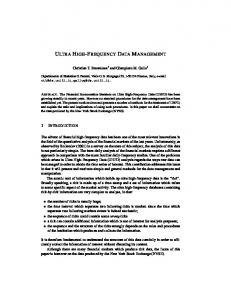
b is the survival function fitted to the ACD data. In this case, the GCS residual where S(·) is unit exponential distributed, EXP(1) in short, regardless the ACD model specification; see Bhatti (2010). Figure 1 displays the QQ plots with simulated envelope of the GCS residual for the ACD models considered in Table III. This figure indicates that in the BSACD model, the

GCS residual shows a good agreement with the EXP(1) distribution, that is, the BSACD model seems to be correctly specified. The same behaviour is not observed for the other models. Table III: ML estimates (with SE in parentheses) and model selection measures for fit to the BASF-SE data. Other ACD models BUACD WEACD GGACD 0.0779 0.0660 0.0724 (0.0203) (0.0177) (0.0183) [< 0.0001] [< 0.0001] [< 0.0001] 0.7077 0.6804 0.7204 0.1010 (0.1181) (0.0936) [< 0.0001] [< 0.0001] [< 0.0001] 0.1051 0.0933 0.0494 0.0213 (0.0201) (0.0117) [< 0.0001] [< 0.0001] [< 0.0001]

4488.384 4516.851 0.7964 0.4344

4461.66 4484.43 0.6238 0.2403

2 0 2

4

6

8

6505.187 6482.413 0.9472 0.7028

6782.066 6753.599 0.8662 0.6887

8 6

empirical quantile

10 empirical quantile

8 6 4 0 0

3

10

4637.567 4660.341 0.9468 0.3410

2

empirical quantile

1.0675 (0.0161)

4

4556.255 4584.722 0.8167 0.3162

1.1974 (0.0180)

10

AIC BIC Q(4) Q(16)

1.0244 (0.0163)

0.2467 (0.0547) 15.0013 (6.5247)

2

ξ

0.4332 (0.0627) 1.3121 (0.0426)

0

φ

8

β

6

α

4

̟

Log-symmetric ACD models BSACD LNACD LtACD −0.2756 −0.2666 −0.2278 (0.0975) (0.0799) (0.0592) [0.0047] [0.0008] [0.0001] 0.5800 0.5951 0.6498 (0.1758) (0.1502) (0.1193) [0.0009] [< 0.0001] [< 0.0001] 0.0403 0.0494 0.0561 (0.0106) (0.0117 ) (0.0124) [0.0001] [< 0.0001] [< 0.0001]

0

theoretical quantile

2

4

6

8

0

theoretical quantile

4

6

8

theoretical quantile

(b) WEACD

(c) GGACD

2

4

6

theoretical quantile

(d) BSACD

8

10 8 6 2 0

2 0

0 0

4

empirical quantile

10 8 6 4

empirical quantile

8 6 4 2

empirical quantile

10

12

(a) BUACD

2

0

2

4

6

theoretical quantile

(e) LNACD

8

0

2

4

6

8

theoretical quantile

(f) LtACD

Figure 1: QQ plot and its envelope for the GCS residuals in the indicated model with the BASF-SE data.

5 Concluding remarks We have discussed a new class of autoregressive conditional duration models based on the log-symmetric distributions, which are based on the conditional median duration. We have presented inference about the model parameters. We have applied the proposed models to a real-world data set of financial transactions of BASF-SE stock on 19th April 2016 from the Dukascopy site. In general, the considered goodness-of-fit measure suggested that the logsymmetric ACD model based on the Birnbaum-Saunders distribution (BSACD) has a better performance. As part of future research, it would be of interest to propose an outlier detection procedure to detect and estimate outlier effects for these models; see Chiang & Wang (2012). Work on these issues is currently in progress and we hope to report some findings in a future paper. References Bauwens, L. & Giot, P. (2000), ‘The logarithmic ACD model: An application to the bid-ask ´ quote process of three NYSE stocks’, Annales d’Economie et de Statistique 60, 117–149. Belfrage, M. (2015), ‘R package ACDm: Tools for autoregressive conditional duration model’, https://cran.r-project.org/web/packages/ACDm. Bhatti, C. (2010), ‘The Birnbaum-Saunders autoregressive conditional duration model’, Mathematics and Computers in Simulation 80, 2062–2078. Birnbaum, Z. W. & Saunders, S. C. (1969), ‘A new family of life distributions’, Journal of Applied Probability 6, 319–327. Chiang, M.-H. (2007), ‘A smooth transition autoregressive conditional duration model’, Studies in Nonlinear Dynamics and Econometrics 11, 108–144. Chiang, M.-H. & Wang, L.-M. (2012), ‘Additive outlier detection and estimation for the logarithmic autoregressive conditional duration model’, Communications in Statistics: Simulation and Computation 41, 287–301. Crow, E. L. & Shimizu, K. (1988), Lognormal Distributions: Theory and Applications, Dekker, New York, US. De Luca, G. & Zuccolotto, P. (2006), ‘Regime-switching Pareto distributions for ACD models’, Computational Statistics and Data Analysis 51, 2179–2191. D´ıaz-Garc´ıa, J. & Leiva, V. (2005), ‘A new family of life distributions based on elliptically contoured distributions’, Journal of Statistical Planning and Inference 128, 445–457. Engle, R. F. (2000), ‘The econometrics of ultra-high-frequency data’, Econometrica 68, 1–22. Engle, R. & Russell, J. (1998), ‘Autoregressive conditional duration: A new method for irregularly spaced transaction data’, Econometrica 66, 1127–1162. Fang, K. T., Kotz, S. & Ng, K. W. (1990), Symmetric Multivariate and Related Distributions, Chapman and Hall, London, UK.

Fernandes, M. & Grammig, J. (2006), ‘A family of autoregressive conditional duration models’, Journal of Econometrics 130, 1–23. Grammig, J. & Maurer, K. (2000), ‘Non-monotonic hazard functions and the autoregressive conditional duration model’, The Econometrics Journal 3, 16–38. Johnson, N., Kotz, S. & Balakrishnan, N. (1994), Continuous Univariate Distributions, Vol. 1, Wiley, New York, US. Johnson, N., Kotz, S. & Balakrishnan, N. (1995), Continuous Univariate Distributions, Vol. 2, Wiley, New York, US. Jones, M. C. (2008), ‘On reciprocal symmetry’, Journal of Statistical Planning and Inference 138, 30393043. Leiva, V., Saulo, H., Le˜ao, J. & Marchant, C. (2014), ‘A family of autoregressive conditional duration models applied to financial data’, Computational Statistics and Data Analysis 79, 175–191. Marshall, A. & Olkin, I. (2007), Life Distributions, Springer, New York, US. Meitz, M. & Terasvirta, T. (2006), ‘Evaluating models of autoregressive conditional duration’, Journal of Business and Economic Statistics 24, 104–12. Mittelhammer, R. C., Judge, G. G. & Miller, D. J. (2000), Econometric Foundations, Cambridge University Press, New York, US. Ng, H. K. T., Kundu, D. & Balakrishnan, N. (2003), ‘Modified moment estimation for the two-parameter Birnbaum-Saunders distribution’, Computational Statistics and Data Analysis 43, 283–298. Pacurar, M. (2008), ‘Autoregressive conditional durations models in finance: A survey of the theoretical and empirical literature’, Journal of Economic Surveys 22, 711–751. Podlaski, R. (2008), ‘Characterization of diameter distribution data in near-natural forests using the Birnbaum-Saunders distribution’, Canadian Journal of Forest Research 18, 518–527. Rieck, J. & Nedelman, J. (1991), ‘A log-linear model for the Birnbaum-Saunders distribution’, Technometrics 3, 51–60. Saulo, H., Leao, J., Leiva, V. & Aykroyd, R. G. (2017), ‘Birnbaum-Saunders autoregressive conditional duration models applied to high-frequency financial data’, Statistical Papers pp. doi:10.1007/s00362–017–0888–6. Vanegas, L. H. & Paula, G. A. (2015), ‘A semiparametric approach for joint modeling of median and skewness’, Test 24(1), 110–135. Vanegas, L. & Paula, G. (2016a), ‘An extension of log-symmetric regression models: R codes and applications’, Journal of Statistical Simulation and Computation 86, 1709–1735. Vanegas, L. & Paula, G. (2016b), ‘Log-symmetric distributions: statistical properties and parameter estimation’, Brazilian Journal of Probability and Statistics 30, 196–220.

Vanegas, L. & Paula, G. (2016c), ‘Log-symmetric regression models under the presence of non-informative left-or right-censored observations’, Test pp. 1–24. Xu, Y. (2013), ‘The lognormal autoregressive conditional duration (LNACD) model and a comparison with an alternative ACD models’, Available at SSRN: https://ssrn.com/abstract=2382159 or http://dx.doi.org/10.2139/ssrn.2382159 . Zhang, M., Russell, J. & Tsay, R. (2001), ‘A nonlinear autoregressive conditional duration model with applications to financial transaction data’, Journal of Econometrics 104, 179– 207. Zheng, Y., Li, Y. & Li, G. (2016), ‘On Fr´echet autoregressive conditional duration models’, Journal of Statistical Planning and Inference 175, 51–66.