Vast volatility matrix estimation for high-frequency financial data - arXiv

arXiv:1002.4754v1 [math.ST] 25 Feb 2010

The Annals of Statistics 2010, Vol. 38, No. 2, 943–978 DOI: 10.1214/09-AOS730 c Institute of Mathematical Statistics, 2010

VAST VOLATILITY MATRIX ESTIMATION FOR HIGH-FREQUENCY FINANCIAL DATA By Yazhen Wang1 and Jian Zou University of Wisconsin-Madison and University of Connecticut High-frequency data observed on the prices of financial assets are commonly modeled by diffusion processes with micro-structure noise, and realized volatility-based methods are often used to estimate integrated volatility. For problems involving a large number of assets, the estimation objects we face are volatility matrices of large size. The existing volatility estimators work well for a small number of assets but perform poorly when the number of assets is very large. In fact, they are inconsistent when both the number, p, of the assets and the average sample size, n, of the price data on the p assets go to infinity. This paper proposes a new type of estimators for the integrated volatility matrix and establishes asymptotic theory for the proposed estimators in the framework that allows both n and p to approach to infinity. The theory shows that the proposed estimators achieve high convergence rates under a sparsity assumption on the integrated volatility matrix. The numerical studies demonstrate that the proposed estimators perform well for large p and complex price and volatility models. The proposed method is applied to real highfrequency financial data.

1. Introduction. Intra-day data observed on the prices of financial assets are often referred to as high-frequency financial data. Advances in technology make high-frequency financial data widely available nowadays for a host of different financial instruments on markets of all locations and at various scales, from individual bids to buy and sell, to the full distribution of such bids. The wide availability, in turn, stirs up an increasing demand for better modeling and statistical inference regarding the price and Received October 2008; revised June 2009. Supported in part by NSF Grant DMS-05-04323, and this material was based on work supported by the National Science Foundation while author was working at the Foundation as a Program Director. AMS 2000 subject classifications. Primary 62H12; secondary 62G05, 62M05, 62P20. Key words and phrases. Convergence rate, diffusion, integrated volatility, matrix norm, micro-structure noise, realized volatility, regularization, sparsity, threshold. 1

This is an electronic reprint of the original article published by the Institute of Mathematical Statistics in The Annals of Statistics, 2010, Vol. 38, No. 2, 943–978. This reprint differs from the original in pagination and typographic detail. 1

2

Y. WANG AND J. ZOU

volatility dynamics of the assets. Diffusion processes are often employed to model high-frequency financial data, and various methodologies have been developed in past several years to estimate integrated volatility (or diffusion variance) over a period of time, say, a day. For a single asset, estimators of integrated volatility include realized volatility (RV) [Andersen et al. (2003), Barndorff-Nielsen and Shephard (2002)], bi-power realized variation (BPRV) [Barndorff-Nielsen and Shephard (2006)], two-time scale realized volatility (TSRV) [Zhang, Mykland and A¨ıt-Sahalia (2005)], multiple-time scale realized volatility (MSRV) [Zhang (2006)], wavelet realized volatility (WRV) [Fan and Wang (2007)], kernel realized volatility (KRV) [Barndorff-Nielsen et al. (2008a)], pre-averaging realized volatility [Jacod et al. (2007)] and Fourier realized volatility (FRV) [Mancino and Sanfelici (2008)]. For multiple assets, we encounter a so-called non-synchronization problem which refers to as the fact that transactions for different assets often occur at distinct times, and the high-frequency prices of the assets are recorded at mismatched time points. Hayashi and Yoshida (2005) and Zhang (2007) have proposed to estimate integrated co-volatility of two assets based on overlap intervals and previous ticks. Barndorff-Nielsen and Shephard (2004) considered estimation of integrated co-volatility for synchronized high-frequency data. A large number of assets are usually involved with in asset pricing, portfolio allocation, and risk management. One key problem we face is to estimate an integrated volatility matrix of large size for the assets. The scenario fits in to the so-called small n and large p or large n but much larger p problem, a current hot topic in statistics. The existing volatility estimation methods work well only for the cases of a single asset or a small number of assets where volatility is either scalar or a small matrix. Their poor behaviors for a large volatility matrix are indicated by random matrix theory and large covariance matrix estimation. Although idealized, the following example is still able to illustrate the point. Consider p assets over unit time interval with all prices following independent Black-Scholes model with zero drift and unit volatility. Then the log prices obey independent standard Brownian motions, and the true integrated volatility matrix Γ is equal to the identity matrix Ip . Assume that we observe all p prices without noise at the same time grids tℓ = ℓ/n for ℓ = 0, 1, . . . , n. The corresponding returns are i.i.d. normal random variables with mean zero and variance 1/n. For b with the following this case, the existing best estimator of Γ is the RV, Γ, representation: n 1X b b b Γ = (Γij ), Γij = Ziℓ Zjℓ for 1 ≤ i, j ≤ p n ℓ=1

where Ziℓ , ℓ = 1, . . . , n, i = 1, . . . , p, are independent N (0, 1) random varib is a poor estimator of Γ when both n and ables. It is widely known that Γ

VOLATILITY MATRIX ESTIMATION

3

p are large [Johnstone (2001), Johnstone and Lu (2009), El Karoui (2007, 2008), Bickel and Levina (2008a, 2008b)]. In fact, for n and p both going to b asymptotically behaves like infinity but p/n → c, the largest eigenvalue of Γ √ 2 (1 + c) while all true eigenvalues are equal to 1. This paper develops a methodology for estimating large volatility matrices based on high-frequency financial data. We establish asymptotic theory for the proposed estimators under sparsity or decay assumptions on integrated volatility matrices as both n and p go to infinity. The estimators proposed in this paper are constructed as follows. In stage one we select grids as pre-sampling frequencies, construct a realized volatility matrix using previous tick method according to each pre-sampling frequency and then take the average of the constructed realized volatility matrices as the stage one estimator, which we call the ARVM estimator. In stage two we regularize the ARVM estimator to yield good consistent estimators of the large integrated volatility matrix. We consider two regularizations: thresholding and banding, developed by Bickel and Levina (2008a, 2008b) in the context of covariance matrix estimation. Thresholding a matrix is to retain only the elements whose absolute values exceed a given value which is called threshold and to replace the others by zero. Thresholding technique was introduced in wavelet literature for function estimation and image analysis [Wang (2006)] where a function is known to have sparse representations in the sense that there are a relatively small number of important terms in its representations, but neither the number nor the locations of the important terms are known. We use thresholding to pick up the important terms for constructing estimators. For a sparse matrix, the small number of elements with large values are important. We need to locate those elements and estimate their values. The thresholding ARVM estimator is designed to find its elements of large magnitude along with their locations. “Banding” a matrix is to keep only the elements in a band along its diagonal and replace others by zero. Banding is analog to smoothing in nonparametric function estimation where in Taylor or orthogonal expansions of a given function, the locations of important terms are known. We simply choose the important terms for building estimators. For a matrix with elements decaying away from its diagonal, important terms are elements within a band along the diagonal, and banding ARVM estimator is used to select its elements within the band. The regularized ARVM estimators provide better volatility estimation that can greatly enhance portfolio allocation and risk management. With the volatility matrix estimators obtained from high-frequency data, we are able to investigate volatility dynamics directly and significantly improve volatility forecasting. See Andersen, Bollerslev and Diebold (2004) and Wang, Yao and Zou (2008).

4

Y. WANG AND J. ZOU

We have shown that for a sparse integrated volatility matrix, the thresholded ARVM estimator not only consistently estimates the integrated volatility matrix but also achieves a high convergence rate when p is allowed to grow as fast as a power of sample size with the power depending on the number of moments imposed on volatility processes and micro-structure noise. When it is known that the integrated volatility matrix has elements decaying away from its diagonal, the banded ARVM estimator is consistent and may enjoy a slightly higher convergence rate than the thresholded ARVM estimator. We have conducted extensive simulation studies for sophisticated price and volatility models with large p. The simulation studies demonstrate that the proposed estimators perform well for finite p and sample size. The proposed method is applied to high-frequency data on 630 stocks traded in the Shanghai Stock Exchange. The problem considered in this paper is much more complex than covariance matrix estimation, and our technical analyses rely on delicate treatments of diffusion processes and noise. Consequently the assumptions imposed and convergence rates obtained are different from those in the covariance matrix context. First, because of micro-structure noise in highfrequency financial data, true assets’ prices are not directly observable; second, observations for continuous price processes are available only at discrete time points; third, price data on multiple assets are nonsynchronized; fourth, randomness in the observed data is caused by micro-structure noise as well as uncertainties in price and volatility processes. Because of noise, nonsynchronization and discretization, the convergence rates for volatility matrix estimation depend on sample size through a rate slower than the usual square root rate for covariance matrix estimation. Due to the multiple random sources in the data, for commonly used price and volatility models, the observed data cannot be sub-Gaussian. As a result, the convergence rates increase in p faster for volatility matrix estimation than for covariance matrix estimation. The rest of the paper is organized as follows. Section 2 introduces the basic models for high-frequency data and the estimation problem. The proposed methodology is presented in Section 3. The asymptotic theory is established in Section 4. Numerical studies are reported in Section 5. All proofs are relegated in Sections 6 and 7. 2. The set-up. 2.1. Observed data. Consider p assets, and let Xi (t) be the true log price at time t of the ith asset, i = 1, . . . , p. Suppose that we have high-frequency data for which the true log price of the ith asset is observed at times tiℓ , ℓ = 1, . . . , ni , and denote by Yi (tiℓ ) the observed log price of the ith asset at time tiℓ . Because of the nonsynchronization problem, typically tiℓ 6= tjℓ for

5

VOLATILITY MATRIX ESTIMATION

any i 6= j. The high-frequency data are usually contaminated with microstructure noise in the sense that the observed log price Yi (tiℓ ) is a noisy version of the corresponding true log price Xi (tiℓ ). It is common to assume (1)

Yi (tiℓ ) = Xi (tiℓ ) + εi (tiℓ ),

i = 1, . . . , p, ℓ = 1, . . . , ni ,

where εi (tiℓ ), i = 1, . . . , p, ℓ = 1, . . . , ni are independent noises with mean zero, for each fixed i, εi (tiℓ ), ℓ = 1, . . . , ni are i.i.d. random variables with variance ηi , and εi (·) and Xi (·) are independent. In the realized volatility literature, it is often assumed that micro-structure noise is i.i.d. and independent of the underlying price process. The simplistic assumption is used to study the effect of micro-structure noise on the volatility estimation. Recently Hansen and Lunde (2006) and Kalnina and Linton (2008), among others, have considered univariate micro-structure models where micro-structure noise has serial correlation and is correlated with the underlying price process. 2.2. Price model. Let X(t) = (X1 (t), . . . , Xp (t))T be the vector of the true log prices at time t of p assets. Following finance theory we assume that X(t) obeys a continuous-time diffusion model, (2)

dX(t) = µt dt + σ Tt dBt ,

t ∈ [0, 1],

where µt = (µ1 (t), . . . , µp (t))T is a drift vector, Bt = (B1t , . . . , Bpt )T is a standard p-dimensional Brownian motion [i.e., Bit are independent standard Brownian motions] and σ t is a p by p matrix. The volatility of X(t) is given by γ(t) = (γij (t))1≤i,j≤p = σ Tt σ t , and its quadratic variation is equal to  Z t Z t γij (s) ds γ(s) ds = [X, X]t = 0

0

, 1≤i,j≤p

Our goal is to estimate the integrated volatility matrix,  Z 1 Z 1 γij (t) dt γ(t) dt = Γ = (Γij )1≤i,j≤p = 0

0

t ∈ [0, 1].

, 1≤i,j≤p

based on noisy and nonsynchronized observations Yi (tiℓ ), ℓ = 1, . . . , ni , i = 1, . . . , p.

6

Y. WANG AND J. ZOU

3. Estimation methodology. 3.1. Realized volatility matrix. Fix an integer m and take τr , r = 1, . . . , m, to be the pre-determined sampling frequency. Let τ = {τr , r = 1, . . . , m}. For asset i, define previous-tick times τi,r = max{tiℓ ≤ τr , ℓ = 1, . . . , ni },

r = 1, . . . , m.

Based on τ we define realized co-volatility between assets i and j by (3)

b ij (τ ) = Γ

m X [Yi (τi,r ) − Yi (τi,r−1 )][Yj (τj,r ) − Yj (τj,r−1 )], r=1

and realized volatility matrix by

b ) = (Γ b ij (τ )). Γ(τ

(4)

The pre-determined sampling frequency τ is usually selected as regular grids. For a fixed m, there are K = [n/m] classes of nonoverlap regular grids given by τ k = {r/m, r = 1, . . . , m} + (k − 1)/n = {r/m + (k − 1)/n, r = 1, . . . , m},

(5) where k = 1, . . . , K and n is the average sample size p

n=

1X ni . p i=1

τ k,

For each sampling frequency using (3) and (4) we define realized cok b b k ). volatility Γij (τ ) between assets i and j and realized volatility matrix Γ(τ Define (6)

K X b ij = 1 b ij (τ k ), Γ Γ K k=1

K X b = (Γ b ij ) = 1 b k ). Γ Γ(τ K k=1

Like TSRV in the univariate case [Zhang, Mykland and A¨ıt-Sahalia (2005)], b is the average of K realized volatility matrices Γ(τ b k ). We use τ k to subΓ b k ) and then take their average to define Γ. b sample data for computing Γ(τ The purpose of subsampling and averaging is to handle noise and yield a better estimator. b to account for the noise We need to adjust the diagonal elements of Γ variances. Set η = diag(η1 , . . . , ηp ) where ηi is the variance of noise εi (tiℓ ). We estimate ηi by n

(7)

ηbi =

i 1 X [Yi (ti,ℓ ) − Yi (ti,ℓ−1 )]2 , 2ni

ℓ=1

VOLATILITY MATRIX ESTIMATION

7

b = diag(b and denote by η η1 , . . . , ηbp ) the estimator of η. Define an estimator of Γ by ˜ = (Γ ˜ ij ) = Γ b − 2mb (8) Γ η,

bij for i 6= j and Γ b ii − 2mb that is, we estimate element Γij of Γ by Γ ηi for ˜ are equal to TSRV of Zhang, Mykland i = j. The diagonal elements of Γ ˜ the averaging realized volatility matrix and A¨ıt-Sahalia (2005). We call Γ (ARVM) estimator. High-frequency financial data are usually not equally spaced nor synchronized, and thus observations may be more or less dense for some assets than others or in some time intervals than others. An asset may have no observation between two consecutive time points in a sampling frequency; then the term involving these two consecutive time points in (3) is equal to zero, and from (6) we can see that the ARVM estimator automatically adjust for data with varying denseness. ˜ provides a good esti3.2. Regularize ARVM estimator. For small p, Γ ˜ has a poor performance when p gets very large. It mator for Γ. However, Γ is well known that even for constant γ(t), when n and p both go to infinity, ˜ are inconsistent. In particular, when p is very large, the estimators like Γ ˜ are far from those corresponding to Γ [see eigenvalues and eigenvectors of Γ Bickel and Levina (2008a, 2008b), Johnstone (2001) and Johnstone and Lu (2009)]. ˜ in order to estiWe need to impose some structure on Γ and regularize Γ mate Γ consistently. Following Bickel and Levina (2008a, 2008b) we consider ˜ with banding or threshdecay or sparsity assumptions on Γ and regularize Γ olding as follows. Decay condition: We assume that the elements of Γ decay when moving away from its diagonal, M |Γij | ≤ (9) , 1 ≤ i, j ≤ p, E[M ] ≤ C, 1 + |i − j|α+1 where M is a positive random variable, and C and α are positive generic constants. Sparsity condition: We assume that Γ satisfies

(10)

p X j=1

|Γij |δ ≤ M π(p),

i = 1, . . . , p, E[M ] ≤ C,

where M is a positive random variable, 0 ≤ δ < 1, and π(p) is a deterministic function of p that grows very slowly in p. Examples of π(p) include 1, log p and a small power of p. The case of δ = 0 in (10) corresponds so that each row of Γ has at most M π(p) number of nonzero elements. Decay condition (9) corresponds to a special case of sparsity

8

Y. WANG AND J. ZOU

condition (10) with δ = 1/(α + 1) and π(p) = log p or 1/(α + 1) < δ < 1 and π(p) = 1. The decay condition depends on the order of p assets in the log price vector X(t). As stocks have no natural ordering, the decay condition may not hold for real volatility matrices of stock returns. As a result, for volatility matrix estimation in financial applications, sparsity is much more realistic than the decay assumption. Examples of sparse matrices include block diagonal matrices, matrices with decay elements from diagonal, matrices with relatively small number of nonzero elements in each row or column and matrices obtained by randomly permuting rows and columns of above matrices. For Γ satisfying decay condition (9), its large elements are within a band along its diagonal, and the elements outside the band are negligible. We ˜ by banding, which is to keep only its elements in a band along regularize Γ its diagonal and replace others by zero. Specifically, the definition of banding ˜ is given by Γ ˜ = (Γ ˜ ij 1(|i − j| ≤ b)), Bb [Γ] where b is a banding parameter, and 1(|i−j| ≤ b) is the indicator of {(i, j), |i− ˜ is equal to Γ ˜ ij for |i − j| ≤ b and zero, j| ≤ b}. The (i, j)th element of Bb [Γ] ˜ the BARVM estimator. otherwise. We call Bb [Γ] If Γ satisfies sparsity condition (10), its important elements are those ˜ by whose absolute values are above a certain threshold. We regularize Γ thresholding which is to retain its elements whose absolute values exceed a given value and replace others by zero. Specifically, we define the threshold˜ by ing of Γ ˜ = (Γ ˜ ij 1(|Γ ˜ ij | ≥ ̟)), T̟ [Γ]

˜ is equal to Γ ˜ ij if its where ̟ is threshold. The (i, j)th element of T̟ [Γ] ˜ absolute value is greater or equal to ̟ and zero, otherwise. We call T̟ [Γ] TARVM estimator. Like most of existing co-volatility matrix estimators, we cannot guarantee the positiveness of the ARVM estimator for finite sample. As the banding and thresholding procedures do not resolve the positiveness issue, the BARVM and TARVM estimators may not be positive for a finite sample. Recently Barndorff-Nielsen et al. (2008b) has developed a kernel-based method with refresh sampling time technique to produce a semi-positive co-volatility matrix estimator. The estimator is designed for fixed p and must suffer from the same drawback as the ARVM estimator for large p; it will be interesting to apply the regularization procedures to the semi-positive matrix estimator and investigate their asymptotic behaviors for large p and n. Banding is analog to smoothing in nonparametric function estimation where in the representations of a target function by Taylor or orthogonal

9

VOLATILITY MATRIX ESTIMATION

expansions the locations of important terms in the expansions are known. We simply select those important terms to keep for building estimators. For a matrix with decaying elements from its diagonal, important terms are elements within a band along the diagonal, and banding is used to select the elements within the band. Thresholding is utilized for estimating a function with sparse representations, where we know that there are a relatively small number of important terms in its representations, but neither the number nor the locations of the important terms are known. We use thresholding to pick up the important terms for constructing estimators. For a sparse matrix, all we know is that a relatively small number of the elements with large values essentially matter. We need to locate those elements and estimate their values. Thresholding is designed to find the elements of large magnitude and their locations. For the BARVM and TARVM estimators, we need to select proper values for banding parameter b and threshold ̟ from data. Data-dependent methods for selecting b and ̟ are illustrated at the end of Section 5.3 for simulated data and at the beginning of Section 5.5 for real data. 4. Asymptotic theory. First we fix some notations for the theoretical analysis. Given a p-dimensional vector x = (x1 , . . . , xp )T and a p by p matrix U = (Uij ), define their ℓd -norms as follows: !1/d p X d |xi | kxkd = , kUkd = sup{kUxkd , kxkd = 1}, d = 1, 2, ∞. i=1

Then kUk2 is equal to the square root of the largest eigenvalue of UUT , kUk1 = max

1≤j≤p

p X i=1

|Uij |,

kUk∞ = max

1≤i≤p

p X j=1

|Uij |,

and kUk22 ≤ kUk1 kUk∞ . For symmetric U, kUk2 is equal to its largest absolute eigenvalue, and kUk2 ≤ kUk1 = kUk∞ . Next we state some technical conditions. A1: For some β ≥ 2,

max max E[|γii (t)|β ] < ∞,

1≤i≤p 0≤t≤1

max E[|εi (tiℓ )|2β ] < ∞.

1≤i≤p

max max E[|µi (t)|2β ] < ∞,

1≤i≤p 0≤t≤1

10

Y. WANG AND J. ZOU

k . A2: Each of p assets has at least one observation between τrk and τr+1 With n = (n1 + · · · + np )/p, we assume ni ni C1 ≤ min ≤ max ≤ C2 , max max |tiℓ − ti,ℓ−1 | = O(n−1 ), 1≤i≤p n 1≤i≤p n 1≤i≤p 1≤ℓ≤ni

m = o(n). Theorem 1. Under models (1) and (2) and conditions A1 and A2 we have for all 1 ≤ i, j ≤ p, ˜ ij − Γij |β ) ≤ Ceβn , (11) E(|Γ

where C is a generic constant free of n and p, and the convergence rate eβn given below is equal to the sum of terms with powers of n and K = [n/m] which depend on whether the observed data in the model specification have micro-structure noise or not. (1) If there is micro-structure noise in model (1), eβn = (Kn−1/2 )−β + K −β/2 + (n/K)−β/2 + K −β + n−β/2 . Thus with K ∼ n2/3 we have en ∼ n−1/6 . (2) If there is no micro-structure noise [i.e. εi (tiℓ ) = 0 and Yi (tiℓ ) = Xi (tiℓ )] in model (1), eβn = (n/K)−β/2 + K −β + n−β/2 . Thus with K ∼ n1/3 we have en ∼ n−1/3 . Remark 1. The convergence rate en can be attributed to three sources due to noise, nonsynchronization and discrete observations for continuous process X(t). Because of micro-structure noise in high-frequency financial data, true log-price X(t) is not directly observable. Furthermore, as a continuous process, X(t) is observed with noise only at discrete time points. Consequently the convergence rate en is slower than n−1/2 . In fact, the optimal convergence rate for the univariate noise case is n−1/4 ; the nonsynchronization for multiple assets further complicates the problem. The terms in convergence rates eβn given by Theorem 1 can be identified to associate with specific sources as follows. The terms (Kn−1/2 )−β + K −β/2 in eβn are due to noise with K −β + n−β/2 contributed by nonsynchronization. Because X(t) is observed at discrete time points, we need to discretize X(t) and use its discretization to approximate integrated volatility matrix. Term (n/K)−β/2 in eβn is attributed to the approximation error due to the discretization of X(t). These are clearly spelled out by Propositions 1–3 in Section 7 for the proof of Theorem 1. The contributions of the three sources to the convergence rates for TSRV, MSRV, realized co-volatility estimators have been shown in Zhang, Mykland and A¨ıt-Sahalia (2005) and Zhang (2006, 2007).

VOLATILITY MATRIX ESTIMATION

11

Theorem 2. Assume that Γ satisfies sparsity condition (10). Then under models (1) and (2) and conditions A1 and A2, we have ˜ − Γk2 ≤ kT̟ [Γ] ˜ − Γk∞ = OP (π(p)[en p2/β hn,p ]1−δ ), kT̟ [Γ]

where en is given in Theorem 1, ̟ = en p2/β hn,p , and hn,p is any sequence converging to infinity arbitrarily slow with one example hn,p = log log(n ∧ p). Remark 2. The convergence rate in Theorem 2 is nearly equal to π(p)[en × p2/β ]1−δ . Since en ∼ n−1/6 for the noise case and en ∼ n−1/3 for the noiseless case, in order to make en p2/β go to zero, p needs to grow more slowly than nβ/12 for the noise case and nβ/6 for the noiseless case. Theorem 3. Assume that Γ satisfies decay condition (9). Then under models (1) and (2) and conditions A1 and A2, we have that ˜ − Γk2 ≤ kBb [Γ] ˜ − Γk∞ = OP ([en p1/β ]α/(α+1+1/β) ), kBb [Γ]

where we select banding parameter b of order (en p1/β )−1/(α+1+1/β) . Remark 3. For Γ satisfying decay condition (9), the sparsity condition is held with δ = 1/(α + 1) and π(p) = log p. The convergence rate corresponding to Theorem 2 under the sparsity condition has a leading factor of order [en p2/β ]α/(α+1) . Comparing it with the rate in Theorem 3, we conclude that the two convergence rates are quite close for reasonably large β. Remark 4. The convergence rates in Bickel and Levina (2008a, 2008b) for large covariance matrix estimation increase in matrix size p through a power of log p, but the convergence rates in Theorems 2 and 3 grow with p through a power of p. The slower convergence rates here are due to the intrinsic complexity of our problem. The log p factor in the convergence rates of covariance matrix estimation is attributed to Gaussianity or subGaussianity imposed on the observed data. In our set-up, observations Yi (tiℓ ) from model (1) have random sources from both micro-structure R t T noise εi (tiℓ ) and true log price X(t) given by model (2). The term 0 σs dBs in X(t) does not obey sub-Gaussianity for common price and volatility models. Even though we assume normality on εi (tiℓ ), the observed data Yi (tiℓ ) cannot be sub-Gaussian for the price and volatility models. Consequently we employ realistic moment conditions in assumption A1, obtain convergence rates for ˜ in Theorem 1 and derive subsequent convergence rates the elements of Γ ˜ in Theorems 2 and 3. with a power of p for the regularized Γ Remark 5. For Gaussian observations, Cai, Zhang and Zhou (2008) have established optimal convergence rates for estimating a covariance matrix which is assumed to belong to a class of matrices satisfying the decay

12

Y. WANG AND J. ZOU

condition. The convergence rate for the minimax risk based on the squared ℓ2 norm is equal to the minimum of n−2α/(2α+1) + log p/n and p/n. The result indicates that the convergence rate in Bickel and Levina (2008a) is suboptimal. It is very interesting and challenging to find optimal convergence rates for the volatility matrix estimation problem in our set-up. 5. Numerical studies. 5.1. High-frequency data. The real data set for our numerical studies is high-frequency tick by tick price data on 630 stocks traded in the Shanghai Stock Exchange over 177 days in 2003. For each day, we computed the ˜ defined in Section 3 where the preARVM estimator corresponding to Γ determined sampling frequencies were selected to correspond with 5 minute returns. This yielded 177 matrices of size 630 by 630 as ARVM estimators of integrated volatility matrices over the 177 days. The average of these 177 matrices was then evaluated and denoted by Θ. 5.2. The simulation model. In our simulation study the true log price X(t) of p assets is generated from model (2) with zero drift, namely, the diffusion model, dX(t) = σTt dBt ,

(12)

t ∈ [0, 1],

where Bt = (B1t , . . . , Bpt )T is a standard p-dimensional Brownian motion, and we take σ t as a Cholesky decomposition of γ(t) = (γij (t))1≤i,j≤p which is defined below. Given the diagonal elements of γ(t), we define its off-diagonal elements by q γij (t) = {κ(t)}|i−j| γii (t)γjj (t), (13) 1 ≤ i 6= j ≤ p, where process κ(t) is given by (14) (15) 0 Wκ,t

κ(t) = Wκ,t =

e2u(t) − 1 , e2u(t) + 1 √

0 0.96Wκ,t

du(t) = 0.03[0.64 − u(t)] dt + 0.118u(t) dWκ,t , − 0.2

p X

√ Bit / p;

i=1

is a standard 1-dimensional Brownian motion independent of Bt . Model (14) is taken from Barndorff-Nielsen and Shephard (2002, 2004). The diagonal elements of γ(t) are generated from four common stochastic volatility models with leverage effect. The four volatility processes are geometric Ornstein–Uhlenbeck processes, the sum of two CIR processes [Cox, Ingersoll and Ross (1985) and Barndorff-Nielsen and Shephard (2002)], the volatility process in Nelson’s GARCH diffusion limit model [Wang (2002)]

13

VOLATILITY MATRIX ESTIMATION

and two-factor log-linear stochastic volatility process [Huang and Tauhen 1 , . . . , U 1 )T and U2 = (U 2 , . . . , U 2 )T be (2005)]. Specifically, let U1t = (U1t pt pt t 1t two independent standard p-dimensional Brownian motions which are in0 , and then define two p-dimensional Brownian dependent of Bt and Wκ,t 1 )T and W2 = (W 2 , . . . , W 2 )T , by 1 1 motions, Wt = (W1t , . . . , Wpt pt t 1t q q (16) Wit2 = ρi Bit + 1 − ρ2i Uit2 , Wit1 = ρi Bit + 1 − ρ2i Uit1 , where we choose the following negative values for ρi to reflect the leverage effect,  −0.62, 1 ≤ i ≤ p/4,    −0.50, p/4 < i ≤ p/2, ρi =  −0.25, p/2 < i ≤ 3p/4,   −0.30, 3p/4 < i ≤ p.

We generate γii (t) as follows.

(1) For 1 ≤ i ≤ p/4, γii (t) are drawn from the geometric Ornstein–Uhlenbeck model driving by Wit1 [Barndorff-Nielsen and Shephard (2002)], (17)

d log γii (t) = −0.6(0.157 + log γii (t)) dt + 0.25 dWit1 .

(2) For p/4 < i ≤ p/2, γii (t) are drawn from the sum of two CIR processes [Barndorff-Nielsen and Shephard (2002)], (18)

γii (t) = 0.98(v1,t + v2,t ),

where v1,t and v2,t obey two CIR models driving by Wit1 and Wit2 , respectively, √ 1 (19) dv1,t = 0.0429(0.108 − v1,t ) dt + 0.1539 v1,t dWi,t , √ 2 (20) . dv2,t = 3.74(0.401 − v2,t ) dt + 1.4369 v2,t dWi,t

(3) For p/2 < i ≤ 3p/4, γii (t) are drawn from the volatility process in Nelson’s GARCH diffusion limit model driving by Wit1 [Barndorff-Nielsen and Shephard (2002)], (21)

1 dγii (t) = [0.1 − γii (t)] dt + 0.2γii (t) dWi,t .

(4) For 3p/4 < i ≤ p, γii (t) are drawn from the two-factor log-linear stochastic volatility model driving by Wit1 and Wit2 [Huang and Tauhen (2005)], (22) where

γii (t) = e−6.8753 s-exp(0.04v1,t + 1.5v2,t − 1.2), 1 dv1,t = −0.00137v1,t dt + dWi,t ,

2 dv2,t = −1.386v2,t dt + (1 + 0.25v2,t ) dWi,t ,  u e , s-exp(u) = 8.5{1 − log(8.5) + u2 / log(8.5)}1/2 ,

(23)

if u ≤ log(8.5), if u > log(8.5).

14

Y. WANG AND J. ZOU

With γii (t) generated from above stochastic differential equations, we multiply γii (t) by 1000θi where θi are the ordered (from the largest to the smallest) diagonal elements of Θ defined in Section 5.1 as the average of 177 daily ARVM estimators for the high-frequency data from the Shanghai market. The adjustment is to roughly match simulated γii (t) with the magnitudes of the diagonal elements of the ARVM estimators for the stock data. Finally the high-frequency data Yi (tiℓ ) are simulated from model (1) with noise εi (tiℓ ) drawing from independent normal distributions √with mean zero √ √ and standard deviation of three choices: 0.002 θi , 0.127 θi and 0.2 θi which correspond to low, medium and high noise levels. The standard deviation is chosen to reflect the empirical fact that relative noise level found in high frequency data typically ranges from 0.001% to 0.01% with 0.001% for individual stock and 0.01% for stock index. In our simulated example, the average volatility is around 1000θi , and thus the three noise standard deviations are translated into 0.002%, 0.004% and 0.065% of the average volatility or relative noise level, respectively. 5.3. The simulation procedure. We need to simulate n values for the price and volatility processes at tℓ = ℓ/n, ℓ = 1, . . . , n. The procedure begins with the generation of matrices γ(tℓ ). First we use normalized partial sums of i.i.d. standard normal random variables to simulate four indepen0 dent Brownian motions, a standard one-dimensional Brownian motion Wκ,t ℓ and three standard p-dimensional Brownian motions, Btℓ , U1tℓ and U2tℓ , and compute Wκ,tℓ , Wt1ℓ and Wt2ℓ according to (15) and (16). We then use the Euler scheme to simulate κ(tℓ ) from (14) with Wκ,tℓ and γii (tℓ ) from (17)– (23) with corresponding components of Wt1ℓ and Wt2ℓ . With available κ(tℓ ) and γii (tℓ ), from (13) we evaluate off-diagonal elements γij (tℓ ), i 6= j. To speed up the simulation of γ(tℓ ) = (γij (tℓ )), we have utilized the following tricks in R programming: (i) group all p diagonal elements γ11 (tℓ ), . . . , γpp (tℓ ) into four vectors of dimension p/4 with each vector drawing from the same volatility model and update each vector in the Euler scheme; (ii) calculate the matrix product of column vector (γ11 (tℓ ), . . . , γpp (tℓ ))T and row vector (γ11 (tℓ ), . . . , γpp (tℓ )) and then take the element by element square root of the obtained matrix; (iii) utilize the Toeplitz matrix operation to evaluate κ(tℓ )i−j ; (iv) use the matrix operation to compute element by element multiplication of the two matrices yielded in steps (ii) and (iii). We take σ tℓ as a Cholesky decomposition of γ(tℓ ) and compute true logprice X(tℓ ) by Xtℓ = Xtℓ−1 + [σ tℓ−1 ]T [Btℓ − Btℓ−1 ]. Finally, data Yi (tℓ ), i = 1, . . . , p, ℓ = 1, . . . , n, are obtained by adding to Xi√ (tℓ ) √ normal √ noise ǫi (tℓ ) of mean zero and standard deviation 0.002 θi , 0.127 θi and 0.2 θi for the cases of low, medium and high noise levels, respectively.

VOLATILITY MATRIX ESTIMATION

15

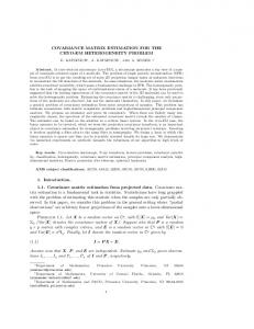
After the simulation has generated volatility matrices γ(tℓ ), log-price values Xi (tℓ ) and synchronized noisy data Yi (tℓ ), i = 1, . . . , p, tℓ = ℓ= Pℓ/n, n 1, . . . , n, we numerically evaluate integrated volatility matrix Γ by ℓ=1 γ(tℓ )/n, ˜ ˜ according to (8) and calculate its banding Bb [Γ] compute ARVM estimator Γ ˜ as described in Section 3.2. Note that there is no and thresholding T̟ [Γ] need to store matrices γ(tℓ ) in the programming loop of ℓ = 1, . . . , n, because at each ℓ step of the loop all we need is to record Xi (tℓ ) and Yi (tℓ ) P and update the partial sum ℓr=1 γ(tr ) to the current step for the purpose of evaluation of Γ by the average of γ(tℓ ) at the end of the loop. Doing so will save huge computer storage space and prevent the simulation program from running out of computer memory. We repeat the whole simulation procedure 500 times. The mean square error (MSE) of a matrix estimator is computed by averaging ℓ2 -norms of the differences between the estimator and Γ over 500 repetitions. We use ˜ Bb [Γ] ˜ and T̟ [Γ] ˜ to evaluate their performances. For estimathe MSEs of Γ, ˜ ˜ tors Bb [Γ] and T̟ [Γ], we select the values of b and ̟ by minimizing their respective MSEs. We generate nonsynchronized data as follows. Instead of generating observations for the processes at n time points, we simulate γ(tℓ ), Xi (tℓ ), Yi (tℓ ), i = 1, . . . , p, at 3n time points tℓ = ℓ/(3n), ℓ = 1, . . . , 3n. Grouping together three consecutive time points we divide the 3n time points tℓ into n groups {t3r−2 , t3r−1 , t3r }, r = 1, . . . , n. For the ith asset, we select one time point at random from each group; from the simulated 3n values of Yi (tℓ ) we choose n values corresponding to the selected time points; we use the n chosen values to form noisy observations for asset i. The selection procedure is applied to p assets for obtaining data on all assets. Because of random selection, the obtained data are nonsynchronized and have n observations Pn for each asset. As in the synchronized case, the true Γ is computed by r=1 γ(t3r )/n. But ˜ Bb [Γ] ˜ and T̟ [Γ], ˜ we use the generated nonsynchronized data to evaluate Γ, where the values of b and ̟ are selected as before by minimizing their respective MSEs. Again we repeat the whole simulation procedure 500 times ˜ Bb [Γ] ˜ and T̟ [Γ] ˜ based on the 500 repetitions. and evaluate MSEs of Γ, 5.4. Simulation results. In the simulations we have tried on different combinations of values for n and p. This section displays the simulation results and reports findings based on n = 200 and p = 512. Figure 1 plots the sample paths of κ(t) corresponding to six initial values κ(0) = 0.537, 0.762, 0.905, 0.964, 0.980, 0.995. The fixed initial values were chosen to obtain various patterns for Γ. The figure shows that process κ(t) is heavily influenced by its initial value, and its whole path stays within a narrow band around the initial value. Figure 2 plots the images of Γ corresponding to these initial values. The image plots indicate that the elements of Γ

16

Y. WANG AND J. ZOU

Fig. 1. Sample path plots for the process κ(t) under different initial values. (a)–(f ) correspond to the sample paths of κ(t) with κ(0) = 0.537, 0.762, 0.905, 0.964, 0.980, 0.995, respectively.

geometrically decay from its diagonal with rate κ(t). The significant elements of Γ fall into a band along its diagonal, and its off-diagonal elements outside the band are negligible. For small κ(t), the decay is very fast, and the band is very narrow. As κ(t) increases, the decay gets slower and slower, and the band becomes wider and wider. As a result, Γ becomes less sparse and is more diffuse along its diagonal. As we will see later, it will be more difficult to estimate Γ. Note that Γ is inhomogeneous, and the band is wider at lower right corner than at upper left corner. This is clearly demonstrated in Figure 2(f) for the case with κ(0) = 0.995.

VOLATILITY MATRIX ESTIMATION

17

Fig. 2. Image plots of matrix Γ generated with different initial values for κ(t). (a)–(f ) correspond to the images of Γ with κ(0) = 0.537, 0.762, 0.905, 0.964, 0.980, 0.995, respectively.

˜ Bb [Γ] ˜ and T̟ [Γ] ˜ are computed over combinations of six The MSEs of Γ, initial values of κ(0), three noise levels and two values of K. The numerical results are summarized in Table 1 for the case of synchronized data. The simulation results indicate that for the given Γ, BARVM estimator has smaller MSE than the corresponding TARVM estimator. This is due to the fact that the decay pattern of Γ is the ideal case for banding. However, if we randomly permute the rows and columns of Γ, the resulting matrix no longer decays along its diagonal but retains the same sparsity. Such a permutation corresponds to a random shuffle of the list of stocks. For each realization matrix of Γ displayed in Figure 2, we take a random permutation

18

Y. WANG AND J. ZOU Table 1 ˜ Bb [Γ] ˜ and T̟ [Γ] ˜ for noisy synchronized data MSEs of Γ, κ(0)

Noise level Low Low Low Low Low Low Medium Medium Medium Medium Medium Medium High High High High High High

Estimator

K

0.537

0.762

0.905

0.964

0.980

0.995

˜ Γ ˜ Γ ˜ Bb [Γ] ˜ T̟ [Γ] ˜ Bb [Γ] ˜ T̟ [Γ] ˜ Γ ˜ Γ ˜ Bb [Γ] ˜ T̟ [Γ] ˜ Bb [Γ] ˜ T̟ [Γ] ˜ Γ ˜ Γ ˜ Bb [Γ] ˜ T̟ [Γ] ˜ Bb [Γ] ˜ T̟ [Γ]

1 5 1 1 5 5 1 5 1 1 5 5 1 5 1 1 5 5

5.595 10.186 0.663 0.845 1.085 1.744 5.641 10.229 0.694 0.871 1.093 1.757 5.769 10.271 0.723 0.896 1.077 1.628

6.039 11.80 1.195 2.456 2.008 3.077 6.097 11.81 1.224 2.466 2.022 3.083 6.234 11.86 1.258 2.429 2.125 3.101

7.511 14.85 3.154 4.595 5.075 6.855 7.649 14.74 2.785 4.101 4.499 7.014 7.717 14.89 3.105 4.043 4.601 6.943

9.959 18.79 6.000 7.457 10.160 12.683 10.479 19.17 6.442 7.680 10.302 12.742 10.521 18.85 6.298 8.765 10.042 12.998

12.259 21.488 8.018 10.928 15.299 18.111 12.280 21.851 9.059 12.058 15.384 19.083 12.942 21.968 10.094 12.844 16.041 19.194

18.270 31.85

18.398 31.95

19.26 33.54

of its rows and columns. Figure 3 plots the images of the obtained matrices. The plot shows that while the significantly large elements are scattered all over the place and the decay patterns completely disappear, the sparsity remains unchanged. For such randomly permuted Γ, the TARVM estimator maintains the same performance, while the BARVM estimator performs very poorly. The simulation results show that the MSEs increase in κ(0). This can be explained by the fact that as κ(0) increases, Γ decays more slowly and becomes less sparse, and thus it is more difficult to estimate Γ. In fact, for κ(0) = 0.995, Γ is so diffuse that banding and thresholding result in almost no reduction in MSEs. In other words, because Γ is not even nearly sparse, ˜ we select almost when applying banding and thresholding procedures to Γ, ˜ all elements in Γ, and the resulting BARVM and TARVM estimators are ˜ Also it is interesting to see that the MSEs increases basically the same as Γ. much faster in κ(0) than in noise level. For the chosen range of κ(0) and the specified noise levels, κ(t) governing the sparsity has more influence on the MSEs than noise. The simulation results suggest that for all three noise levels, the estimators with K = 1 have better performance than with K = 5. We have tried to

VOLATILITY MATRIX ESTIMATION

19

Fig. 3. Image plots of the matrices obtained by randomly permuting rows and columns of Γ in Figure 2. (a)–(f ) correspond to the images of randomly permuted Γ with κ(0) = 0.537, 0.762, 0.905, 0.964, 0.980, 0.995, respectively.

√ increase noise standard deviation up to 0.6 θi and found that for noise √ standard deviation from 0.4 θi on, the estimators with K = 1 perform worse than with K = 5. We have also tried on different values for K and obtained the similar results. Like the TSRV estimator in Zhang, Mykland and A¨ıtSahalia (2005), the role of K is to balance subsampling and averaging in ˜ for the purpose of noise reduction. Its effect is clearly demonstrated by Γ asymptotic analysis as illustrated in Theorem 1 and Remark 1. However, the simulation results imply that it needs large noise to manifest numerically the ˜ benefit of choosing K greater than 1 in the construction of Γ.

20

Y. WANG AND J. ZOU Table 2 ˜ Bb [Γ] ˜ and T̟ [Γ] ˜ for noisy nonsynchronized data MSEs of Γ, κ(0)

Noise level Low Low Low Medium Medium Medium High High High

Estimator

K

0.537

0.762

0.905

0.964

0.980

0.995

˜ Γ ˜ Bb [Γ] ˜ T̟ [Γ] ˜ Γ ˜ Bb [Γ] ˜ T̟ [Γ] ˜ Γ ˜ Bb [Γ] ˜ T̟ [Γ]

1 1 1 1 1 1 1 1 1

12.86 3.305 3.842 12.98 3.911 3.374 13.16 3.443 3.997

16.99 4.778 5.281 17.10 4.834 4.728 17.15 4.776 4.902

27.13 8.718 13.38 27.15 8.759 11.662 27.50 8.779 11.70

48.37 20.375 30.29 48.57 22.49 30.53 48.07 21.946 29.98

68.77 34.29 46.11 69.23 36.04 50.64 71.44 42.23 56.27

152.75 85.10 121.15 153.57 92.70 123.22 151.85 69.27 100.13

˜ Bb [Γ] ˜ and T̟ [Γ] ˜ for noisy nonsynchroTable 2 displays the MSEs of Γ, nized data. The comparison of Tables 1 and 2 shows that the MSEs in Table 2 are much larger than the corresponding ones in Table 1 for all three noise levels and six values of κ(0) considered. The phenomenon suggests that the contribution in MSEs due to nonsynchronization dominates over that due to noise. We note particularly that even for the case of κ(0) = 0.995 where ˜ for the Γ is very diffuse and regularizations have little improvement on Γ synchronization case, regularizations in the non-synchronization case still ˜ with sizable reduction on MSEs. Similar to the synchronized improve Γ case, the estimators with K = 1 have smaller MSEs than with K = 5 for all three noise levels. Since nonsynchronization significantly inflates MSEs, it requires very large noise to manifest numerically the effect on MSE reduc˜ Apart from the phenomenon tion by using K > 1 in the construction of Γ. due to nonsynchronization, Table 2 exhibits the similar MSE patterns as Table 1. 5.5. An application to the stock data. We applied the proposed method to the high-frequency stock price data from the Shanghai market. Denote ˜ i , i = 1, . . . , 177, the daily ARVM estimators obtained in Section 5.1. by Γ ˜ i , we computed its eigenvalues and collected them as a set. For each of Γ ˜ i have wide ranges, with some very big positive The eigenvalue sets for Γ values for the largest eigenvalues and many negative values for the smallest eigenvalues. As stocks have no natural ordering, the decay assumption is not realistic for volatility matrices, and banding may not be appropriate for ˜ i . We regularized Γ ˜ i by thresholding. The threshold ̟i applied to Γ ˜ i was Γ ˜ i . For a ∈ (0, 1), calibrated through the quantiles of the absolute entries of Γ ˜ let ̟i,a be the a-quantile of the absolute entries of Γi . Then we reduced

21

VOLATILITY MATRIX ESTIMATION

threshold selection to the selection of a. Define 176 X ˜ i+1 − T̟ [Γ ˜ i ]k22 . (24) kΓ Λ(a) = i,a i=1

We selected the value of a by minimizing Λ(a) over a ∈ (0, 1). The threshold selection procedure was motivated as follows. Because the ARVM estimators were evaluated at the daily level where stationarity is a reasonable assumption on volatility in financial time series, we predicted one day ahead of the daily realized volatility matrix by the current thresholded daily realized volatility matrix with prediction performance measured by the ℓ2 -norm of the prediction error. Thresholds ̟i,a were then selected by minimizing Λ(a), the sum of the squared ℓ2 -norms of the prediction errors over 176 pairs of consecutive days. Our calculation resulted in selecting 0.95 for a. ˜ i by ̟i,0.95 , namely, for each of Γ ˜ i we retained its top We thresholded Γ 5% entries in magnitude and replaced the rest by zero. We evaluated the ˜ i ]. Thresholding attributes to significantly narrowing eigenvalues of T̟i,0.95 [Γ ˜ i had negative smallest eigenvaldown the eigenvalue ranges. Since many Γ ues, we truncated the negative eigenvalues at zero and plotted in Figure 4 the ˜ i and T̟ ˜ corresponding largest eigenvalues of Γ i,0.95 [Γi ]. The plot shows that the reductions of the largest eigenvalues due to thresholding are over 50% for many days. Since eigen based analyses like clustering analysis, principal component analysis and portfolio allocation are routinely applied in practice, the study indicates that blind applications of such analyses to large realized volatility matrices without regularization may end up with very misleading conclusions. 6. Proofs of Theorems 2 and 3. Denote by C a generic constant whose value is free of n and p and may change from appearance to appearance. OP and oP denote orders in probability as both n and p go to infinity. We will prove Theorem 1 in Section 7. This section assumes (11) in Theorem 1. We use it to establish Theorems 2 and 3 by following Bickel and Levina (2008a, 2008b). Proof of Theorem 3. Using the relationship between ℓ2 - and ℓ∞ norms, triangle inequality, and decaying condition (10), we have ˜ − Γk2 ≤ kBb [Γ] ˜ − Γk∞ kBb [Γ] (25) ˜ − Bb [Γ]k∞ + kBb [Γ] − Γk∞ , ≤ kBb [Γ] (26) (27)

kBb [Γ] − Γk∞ ≤ max

1≤i≤p

X

|i−j|>b

|Γij | ≤ 2M

∞ X

k=b+1

˜ − Bb [Γ]k∞ ≤ (2b + 1) max |Γ ˜ ij − Γij |. kBb [Γ] |i−j|≤b

k−α−1 ≤

2M −α b , α

22

Y. WANG AND J. ZOU

Fig. 4. Plots of the largest eigenvalues of daily realized volatility matrices and the thresholded daily realized volatility matrices for the stock data from the Shanghai market. The solid line represents the largest eigenvalues of daily realized volatility matrices, and the dotted line corresponds to the largest eigenvalues of the thresholded daily realized volatility matrices.

From (11) we get   ˜ ij − Γij | > d P max |Γ |i−j|≤b

≤ ≤

X

|i−j|≤b

˜ ij − Γij | > d) P (|Γ

β p(2b + 1) ˜ ij − Γij |β ] ≤ Cpben . max E[| Γ dβ dβ |i−j|≤b

Combining above probability inequality with (27) we obtain   ˜ − Bb [Γ]k∞ > d) ≤ P max |Γ ˜ ij − Γij | > d/(2b + 1) P (kBb [Γ] |i−j|≤b

(28)

≤

Cpbβ+1 eβn Cb−αβ ≤ , dβ dβ

where the last inequality is due to the fact that for the selected b in the theorem, pbβ+1 eβn ∼ b−αβ .

23

VOLATILITY MATRIX ESTIMATION

Collecting together (25), (26) and (28) and taking d = 2d1 b−α ∼ (peβn )α/(αβ+β+1) ,

we conclude

˜ − Γk∞ > d) ≤ P (kBb [Γ] ˜ − Bb [Γ]k∞ > d1 b−α ) P (kBb [Γ] + P (kBb [Γ] − Γk∞ > d1 b−α )

≤ ≤

C

dβ1 C dβ1

+ P (M > αd1 /2) 2E[M ] → 0, αd1

+

as d1 → ∞.

This completes the proof of Theorem 3.  We need the following lemmas for proving Theorem 2. Lemma 1. Assume that Γ satisfies sparse condition (10) and ̟ is chosen as in Theorem 2. Then for any fixed a > 0, p X (29) max |Γij |1(|Γij | ≤ a̟) ≤ a1−δ M π(p)̟ 1−δ = OP (π(p)̟ 1−δ ), 1≤i≤p

(30)

j=1

max

1≤i≤p

p X j=1

1(|Γij | ≥ a̟) ≤ a−δ M π(p)̟ −δ = OP (π(p)̟ −δ ).

Proof. Simple algebraic manipulation shows p X |Γij |1(|Γij | ≤ a̟) max 1≤i≤p

j=1

1−δ

≤ (a̟)

max

1≤i≤p

p X j=1

|Γij |δ 1(|Γij | ≤ a̟)

≤ a1−δ ̟1−δ M π(p) = OP (π(p)̟ 1−δ )

which proves (29). (30) is proved as follows: max

1≤i≤p

p X j=1

1(|Γij | ≥ a̟) ≤ max

1≤i≤p

p X j=1

[|Γij |/(a̟)]δ 1(|Γij | ≥ a̟)

≤ (a̟)−δ max

1≤i≤p

−δ

≤ (a̟)

p X j=1

|Γij |δ

M π(p) = OP (π(p)̟ −δ ).



24

Y. WANG AND J. ZOU

Lemma 2. Assume that Γ satisfies sparse condition (10), ̟ is chosen as in Theorem 2 and (11) is held. Then ˜ ij − Γij | = OP (en p2/β ) = oP (̟), max |Γ

(31)

1≤i,j≤p

(32)

P

max

1≤i≤p

(33)

max

1≤i≤p

p X j=1

p X j=1

!

˜ ij − Γij | ≥ ̟/2} > 0 1{|Γ

= o(1),

˜ ij | ≥ ̟, |Γij | < ̟) ≤ 2δ M π(p)̟−δ + oP (1) 1(|Γ = OP (π(p)̟ −δ ).

Proof. Taking d = d1 p2/β en , applying the Markov inequality and using (11) we obtain ˜ ij − Γij | > d) ≤ P ( max |Γ 1≤i,j≤p

p X

2 β ˜ ij − Γij | > d) ≤ Cp en = C → 0 P (|Γ dβ dβ1 i,j=1

as n, p → ∞ and then d1 → ∞. This proves (31). Using above inequality we have ! p   X ˜ ij − Γij | ≥ ̟/2} > 0 ≤ P max |Γ ˜ ij − Γij | ≥ ̟/2 1{|Γ P max 1≤i≤p

1≤i,j≤p

j=1

2β Cp2 eβn 2β C ≤ = β →0 ̟β hn,p since hn,p → ∞ as n, p → ∞ which proves (32). To show (33) we employ (30) and (32) to get max

1≤i≤p

p X j=1

˜ ij | ≥ ̟, |Γij | < ̟) ≤ max 1(|Γ

1≤i≤p

p X j=1

+ max

1≤i≤p

≤ max

1≤i≤p

p X j=1

p X j=1

+ max

1≤i≤p

˜ ij | ≥ ̟, |Γij | ≤ ̟/2) 1(|Γ ˜ ij | ≥ ̟, ̟/2 < |Γij | < ̟) 1(|Γ

˜ ij − Γij | ≥ ̟/2) 1(|Γ

p X j=1

1(|Γij | > ̟/2)

VOLATILITY MATRIX ESTIMATION

25

≤ oP (1) + 2δ M π(p)̟−δ

= OP (π(p)̟ −δ ).



Proof of Theorem 2. With the relationship between ℓ2 - and ℓ∞ norms and the triangle inequality, we have ˜ − Γk2 ≤ kT̟ [Γ] ˜ − T̟ [Γ]k2 + kT̟ [Γ] − Γk2 kT̟ [Γ] Lemma 1 implies

˜ − T̟ [Γ]k∞ + kT̟ [Γ] − Γk∞ . ≤ kT̟ [Γ]

kT̟ [Γ] − Γk∞ = max

1≤i≤p

p X j=1

|Γij |1(|Γij | ≤ ̟) = OP (π(p)̟ 1−δ ).

˜ − T̟ [Γ]k∞ is also of order The theorem is proved if we show that kT̟ [Γ] 1−δ ̟ π(p) in probability. Indeed, with simple algebra and Lemmas 1 and 2 we establish it as follows: p X ˜ ij − Γij |1(|Γ ˜ ij | ≥ ̟, |Γij | ≥ ̟) ˜ |Γ kT̟ [Γ] − T̟ [Γ]k∞ ≤ max 1≤i≤p

j=1

+ max

1≤i≤p

+ max

1≤i≤p

p X j=1

p X j=1

˜ ij |1(|Γ ˜ ij | ≥ ̟, |Γij | < ̟) |Γ ˜ ij | < ̟, |Γij | ≥ ̟) |Γij |1(|Γ

˜ ij − Γij | max ≤ max |Γ 1≤i,j≤p

+ max

1≤i≤p

1≤i≤p

p X j=1

p X j=1

|Γij |1(|Γij | < ̟)

˜ ij − Γij | max + max |Γ 1≤i,j≤p

+ ̟ max

1≤i≤p

1(|Γij | ≥ ̟)

1≤i≤p

p X j=1

p X j=1

˜ ij | ≥ ̟, |Γij | < ̟) 1(|Γ

1(|Γij | ≥ ̟)

= oP (̟)OP (π(p)̟ −δ ) + OP (π(p)̟ 1−δ ) + oP (̟)OP (π(p)̟ −δ ) + ̟OP (π(p)̟ −δ ) = OP (π(p)̟1−δ ),

26

Y. WANG AND J. ZOU

where the orders in line five of the six equation array are from (29)–(31) and (33).  7. Proof of Theorem 1. b defined in (6). We decompose Γ b = (Γ b ij ) into 7.1. Decomposition of Γ three parts with 12 terms in this subsection and show that all parts meet condition (11) in next four subsections. Denote by k k Yrk = (Y1 (τ1,r ), . . . , Yp (τp,r ))T ,

k k Xkr = (X1 (τ1,r ), . . . , Xp (τp,r ))T ,

k k εkr = (ε1 (τ1,r ), . . . , εp (τp,r ))T

the vectors formed by data, true log price and noise at time points prior to τr k , . . . , τ k are not equal, these vectors are for all p assets. Note that since τ1,r p,r nonsynchronized in the sense that their coordinates are the corresponding processes evaluated at different time points. From (6), we have K X m X k k b= 1 Γ [Yrk − Yr−1 ][Yrk − Yr−1 ]T K k=1 r=1

=

K m 1 XX k [Xr − Xkr−1 + εkr − εkr−1 ][Xkr − Xkr−1 + εkr − εkr−1 ]T K r=1 k=1

K m 1 XX (34) = {[Xkr − Xkr−1 ][Xkr − Xkr−1 ]T + [εkr − εkr−1 ][εkr − εkr−1 ]T K k=1 r=1

+ [Xkr − Xkr−1 ][εkr − εkr−1 ]T + [εkr − εkr−1 ][Xkr − Xkr−1 ]T }

≡

K m 1 XX k [Xr − Xkr−1 ][Xkr − Xkr−1 ]T + G(1) + G(2) + G(3), K k=1 r=1

where G(1), G(2), G(3) are sums involving with noise components and will be handled in Section 7.2, and the first term corresponds to the average realized volatility estimator based on noiseless nonsynchronized true log prices Xkr which will be decomposed further below. Since Xkr and Xkr−1 k and τ k are evaluated at time points τi,r i,r−1 , and condition A2 indicates k k k k τi,r−1 ≤ τr−1 < τi,r ≤ τr , we insert synchronized true log prices X(τrk ) and k ) in between Xk and Xk X(τr−1 r r−1 and write k k Xkr − Xkr−1 = Xkr − X(τrk ) + X(τrk ) − X(τr−1 ) + X(τr−1 ) − Xkr−1 .

VOLATILITY MATRIX ESTIMATION

27

Using the above expression to expand (Xkr − Xkr−1 )(Xkr − Xkr−1 )T , we obtain the following decomposition of the first term on the right-hand side of (34): K m 1 XX k [Xr − Xkr−1 ][Xkr − Xkr−1 ]T K k=1 r=1

K m 1 XX k k {[X(τrk ) − X(τr−1 )][X(τrk ) − X(τr−1 )]T = K k=1 r=1

+ [Xkr − X(τrk )][Xkr − X(τrk )]T

k k + [X(τr−1 ) − Xkr−1 ][X(τr−1 ) − Xkr−1 ]T k + [Xkr − X(τrk )][X(τr−1 ) − Xkr−1 ]T

k + [X(τr−1 ) − Xkr−1 ][Xkr − X(τrk )]T

k + [Xkr − X(τrk )][X(τrk ) − X(τr−1 )]T

(35)

k + [X(τrk ) − X(τr−1 )][Xkr − X(τrk )]T

k k )]T ) − Xkr−1 ][X(τrk ) − X(τr−1 + [X(τr−1

k k ) − Xkr−1 ]T } )][X(τr−1 + [X(τrk ) − X(τr−1

≡ V + H(1) + · · · + H(8),

where V corresponds to the average realized volatility estimator based on synchronized true log prices X(τrk ), and H(1), . . . , H(8) are contributions due to nonsynchronization in true log prices. Then from (34) and (35) we ˜ −Γ=Γ b − 2mb decompose Γ η − Γ into three parts with 12 terms, ˜ Γ − Γ = [G(1) − 2mb η + G(2) + G(3)] + [V − Γ] (36) + [H(1) + · · · + H(8)].

Propositions 1–3 in Sections 7.2–7.4 below, respectively, establish orders for the βth moments of the three parts on the right-hand side of (36). Putting these order results together and applying the H¨older inequality, we immediately prove Theorem 1. 7.2. Analyze Gs for the effect of micro-structure noise. Let G(1) = (Gij (1)),

G(2) = (Gij (2)),

G(3) = (Gij (3)).

The purpose of this subsection is to show Proposition 1. i, j ≤ p,

Under the assumptions of Theorem 1, we have for 1 ≤

E[|Gij (1) − 2mb ηi 1(i = j) + Gij (2) + Gij (3)|β ] ≤ C[(Kn−1/2 )−β + K −β/2 ].

28

Y. WANG AND J. ZOU

We prove the proposition by deriving the orders for the βth moments of Gij (1) − 2mηi 1(i = j), Gij (2), Gij (3) and 2m(b ηi − ηi ) in Lemmas 3–5 below. Lemma 3. p,

Under the assumptions of Theorem 1, we have for 1 ≤ i, j ≤ E[|Gij (1) − 2mηi 1(i = j)|β ] ≤ C(Kn−1/2 )−β .

Proof. From the definition of G(1) in (34), we have Gij (1) − 2mηi 1(i = j) =

K m 1 XX k k k k [εi (τi,r ) − εi (τi,r−1 )][εj (τj,r ) − εj (τj,r−1 )] − 2ηi 1(i = j) K k=1 r=1

K m 1 XX k k = {εi (τi,r )εj (τj,r ) − ηi 1(i = j) K r=1 k=1

k k + εi (τi,r−1 )εj (τj,r−1 ) − ηi 1(i = j)

k k k k − εi (τi,r )εj (τj,r−1 ) − εi (τi,r−1 )εj (τj,r )}

1 [R1 + R2 − R3 − R4 ]. K k and τ k are equal to some t and t , for fixed i, ε (t ) are Note that τi,r i iℓ iℓ jℓ j,r i.i.d., and for i 6= j, {εi (tiℓ )} and {εj (tjℓ )} are independent. Thus, R1 and R2 are the sums of εi (tiℓ )εj (tjℓ ), R3 is the sum of εi (tiℓ ) multiplying by the lagged εj (tjℓ ), and R4 is the sum of εj (tjℓ ) multiplying by the lagged εi (tiℓ ). As a result, all four Rs are martingales. We apply the Burkholder inequality [Chow and Teicher (1997), Section 11.2] to Rs and use the moment condition on εi (tiℓ ) in condition A1 to obtain ≡

E[|Gij (1) − 2mηi 1(i = j)|β ] ≤ CK −β (Km)β/2−1

m K X X k=1 r=1

k k E{|εi (τi,r )εj (τj,r ) − ηi 1(i = j)|β k k + |εi (τi,r−1 )εj (τj,r−1 ) − ηi 1(i = j)|β

+ |εi (τi,r )εj (τj,r−1 )|β

+ |εi (τi,r−1 )εj (τj,r )|β }

≤ CK −β (Km)β/2 {E[|εi (ti,1 )εj (tj,1 ) − ηi 1(i = j)|β ]

+ E[|εi (ti,1 )|β ]E[|εj (tj,1 )|β ]}

≤ C(m/K)β/2 ≤ C(Kn−1/2 )−β

VOLATILITY MATRIX ESTIMATION

29

which proves the lemma.  Lemma 4. p,

Under the assumptions of Theorem 1, we have for 1 ≤ i, j ≤

E[|Gij (2)|β ] ≤ CK −β/2 ,

E[|Gij (3)|β ] ≤ CK −β/2 .

Proof. Because of similarity, we provide arguments only for the first result. Simple algebra shows that KGij (2) =

K X m X

k k k k [Xi (τi,r ) − Xi (τi,r−1 )][εj (τj,r ) − εj (τj,r−1 )]

m K X X

k k k [Xi (τi,r ) − Xi (τi,r−1 )]εj (τj,r )

k=1 r=1

(37)

=

k=1 r=1

− =

K X m X k=1 r=1

K m−1 X X k=1 r=1

k k k [Xi (τi,r ) − Xi (τi,r−1 )]εj (τj,r−1 )

k k k k )]εj (τj,r ) ) − Xi (τi,r+1 [2Xi (τi,r ) − Xi (τi,r−1

K X k k k + [Xi (τi,m ) − Xi (τi,m−1 )]εj (τj,m ) k=1

−

K X k k k [Xi (τi,1 ) − Xi (τi,0 )]εj (τj,0 ) k=1

≡ R5 + R6 − R7 .

Conditional on the whole path of Xt , R5 , R6 and R7 , all are sums of independent random variables εj (tjℓ ). Thus E[|R5 |β |X] ≤ C(Km)β/2−1 ×

K m−1 X X k=1 r=1

k k k k β |2Xi (τi,r ) − Xi (τi,r−1 ) − Xi (τi,r+1 )|β E[|εj (τj,r )| ]

≤ C(Km)β/2−1

K m−1 X X k=1 r=1

k k k |2Xi (τi,r ) − Xi (τi,r−1 ) − Xi (τi,r+1 )|β .

Taking expectation in above inequality we get E[|R5 |β ] ≤ C(Km)β/2−1

K m−1 X X k=1 r=1

k k k E|2Xi (τi,r ) − Xi (τi,r−1 ) − Xi (τi,r+1 )|β

30

Y. WANG AND J. ZOU β/2−1

≤ C(Km) (38)

K m−1 X X Z E

k τi,r−1

k=1 r=1

k τi,r−1

k=1 r=1

β/2−1

≤ C(Km)

≤ C(Km)β/2−1

K m−1 X X Z E

K m−1 X X

k τi,r

k τi,r

σ i (s) dBs − γii (s) ds +

Z

Z

k τi,r

k τi,r+1 k τi,r

m−β/2 max E|γii (s)|β/2

k=1 r=1

k τi,r+1

β σ i (s) dBs

β/2 γii (s) ds

0≤s≤1

≤ C(Km)β/2 m−β/2 = CK β/2 ,

where the third inequality is due to an application of the Burkholder inequality [He, Wang and Yan (1992), Section 10.5 and Jacod and Shiryaev (2003), Section 7.3] to the stochastic integrals. Similarly, we have K X

k k k |Xi (τi,m ) − Xi (τi,m−1 )|β E[|εj (τj,m )|β ]

K X

k k |Xi (τi,m ) − Xi (τi,m−1 )|β ,

E[|R6 |β ] ≤ CK β/2−1

K X

k k E|Xi (τi,m ) − Xi (τi,m−1 )|β ≤ CK β/2 m−β/2 ,

E[|R7 |β |X] ≤ CK β/2−1

K X

k k k β )| E[|εj (τj,0 )|β ] ) − Xi (τi,0 |Xi (τi,1

K X

k k β |Xi (τi,1 ) − Xi (τi,0 )| ,

E[|R6 |β |X] ≤ CK β/2−1 ≤ CK (39)

≤ CK (40)

β/2−1

k=1

k=1

β/2−1

k=1

k=1

k=1

E[|R7 |β ] ≤ CK β/2 m−β/2 .

Collecting (37)–(40) together, we prove the result for Gij (2).  Lemma 5.

Under the assumptions of Theorem 1, we have for 1 ≤ i ≤ p, E[|m(b ηi − ηi )|β ] ≤ C(Kn−1/2 )−β .

Proof. Taking K = 1 in the proofs of Lemmas 3 and 4, we have that conditional on the whole path of Xi (t), ! ni X β/2 −β β 2β E[|b ηi − ηi | |Xi ] ≤ Cni [Xi (tiℓ ) − Xi (ti,ℓ−1 )] + ni , ℓ=1

31

VOLATILITY MATRIX ESTIMATION

E[|b ηi − ηi | ] ≤

Cn−β i

≤

Cn−β i

β

ni X ℓ=1

ni X

2β

E{[Xi (tiℓ ) − Xi (ti,ℓ−1 )] Cn−β i

β/2 + ni

ℓ=1

!

β/2 } + ni

!

≤ Cn−β/2

which immediately shows the lemma as n = mK.  7.3. Analyze V for average realized volatility based on synchronized true log price. Let m X k k )], [Xi (τrk ) − Xi (τr−1 )][Xj (τrk ) − Xj (τr−1 [Xi , Xj ](k) = (41)

r=1

[X, X](k) = ([Xi , Xj ](k) ),

where [Xi , Xj ](k) is realized co-volatility between Xi (t) and Xj (t) based on true log prices at the same grid times τrk , r = 1, . . . , m, and V is equal to the average of K realized volatility matrices based on synchronized true log prices X(τrk ), r = 1, . . . , m. Then from (35), we have that K 1 X [X, X](k) . V = (Vij ) = K

(42)

k=1

Proposition 2. i, j ≤ p,

Under the assumptions of Theorem 1, we have for 1 ≤ E(|Vij − Γij |β ) ≤ Cm−β/2 .

Proof. Note that K

1 X [Xi , Xj ](k) , K k=1 β K 1 X ([Xi , Xj ](k) − Γij ) |Vij − Γij |β = K Vij =

k=1

≤

K 1 X |[Xi , Xj ](k) − Γij |β . K k=1

Lemma 6 below gives the moment inequality for each [Xi , Xj ](k) , from which we immediately show E(|Vij − Γij |β ) ≤

K 1 X E|[Xi , Xj ](k) − Γij |β K k=1

32

Y. WANG AND J. ZOU

≤ Cm−β/2 .



Lemma 6. Under the assumptions of Theorem 1, we have that for 1 ≤ k ≤ K and 1 ≤ i, j ≤ p, E(|[Xi , Xj ](k) − Γij |β ) ≤ Cm−β/2 . Proof. Note that [X, X](k) is defined by X(τrk ) for r = 1, . . . , m while k is fixed. For fixed k, τrk , r = 1, . . . , m, are equally spaced grids on [0, 1]. As k is fixed throughout the proof of the lemma, to simplify notation we write τrk as τr , r = 1, . . . , m, in the rest of the proof. The effects of diffusion drifts on realized volatility are in high and negligible orders. For simplicity, we assume µt = 0. Observe that [Xi , Xj ](k) − Γij

(43)

Z m X {Xi (τr ) − Xi (τr−1 )}{Xj (τr ) − Xj (τr−1 )} − = m Z X r=1

=

γij (t) dt

0

r=1

=

1

τr

(σ is )T dBs

τr−1

Z

τr τr−1

(σ js )T dBs −

Z

τr

γij (t) dt τr−1



m X {Dir (τr )Djr (τr ) − [Dir , Djr ]τr }, r=1

where σ is = (σ1i,s , . . . , σpi,s)T is the ith column of σs , T

γij (s) = (σ is ) σjs =

p X

σai,s σaj,s ,

a=1

Dir (t) = Xi (τr ) − Xi (τr−1 ) =

Z

t

(σ is )T dBs ,

τr−1

t ∈ [τr−1 , τr )

and Di (t) = Dir (t) for t ∈ [τr−1 , τr ). Applying Itˆo’s lemma, we obtain the following stochastic integral expression: Z τr (44) Dir (τr )Djr (τr ) − [Dir , Djr ]τr = {Dir (s)σ is + Djr (s)σ js }T dBs τr−1

which has quadratic variation Z τr 2 2 (45) {Dir (s)γii (s) + Djr (s)γjj (s) + 2Dir (s)Djr (s)γij (s)} ds. τr−1

VOLATILITY MATRIX ESTIMATION

33

Thus from (43)–(45) we immediately show that [Xi , Xj ](k) −Γij has quadratic variation Z 1 {Di2 (s)γii (s) + Dj2 (s)γjj (s) + 2Di (s)Dj (s)γij (s)} ds (46)

0

≤2

Z

0

1

{Di2 (s)γii (s) + Dj2 (s)γjj (s)} ds,

where the Cauchy–Schwarz inequality is employed to show that |γij (s)|2 ≤ γii (s)γjj (s), and hence 2|Di (s)Dj (s)γij (s)| ≤ Di2 (s)γii (s) + Dj2 (s)γjj (s).

Applying the Burkholder inequality [He, Wang and Yan (1992), Section 10.5 and Jacod and Shiryaev (2003), Section 7.3] to the stochastic integral expression of [Xi , Xj ](k) − Γij given by (43)–(44) and using (44)–(46), we have β/2   Z 1 β 2 2 (k) [Di (s)γii (s) + Dj (s)γjj (s)] ds E{|[Xi , Xj ] − Γij | } ≤ CE 0 (47) Z 1

≤C

0

E{|Di2 (s)γii (s) + Dj2 (s)γjj (s)|β/2 } ds.

On the other hand, simple algebraic manipulations derive the inequalities (48) (49)

|Di2 (s)γii (s) + Dj2 (s)γjj (s)|β/2 ≤ 2β/2−1 {|Di2 (s)γii (s)|β/2

E{|Di2 (s)γii (s)|β/2 }

≤

q

+ |Dj2 (s)γjj (s)|β/2 }, E{|Di (s)|2β }E{|γii (s)|β },

and we apply the Burkholder inequality [He, Wang and Yan (1992), Section 10.5 and Jacod and Shiryaev (2003), Section 7.3] to the stochastic integral Di (s), and obtain β   Z τr 2β γii (s) ds E{|Di (s)| } ≤ C max E 1≤r≤m

(50)

τr−1

≤ C max (τr − τr−1 )β max E{|γii (s)|β } 1≤r≤m

0≤s≤1

≤ Cm−β max E{|γii (s)|β }. 0≤s≤1

Collecting together (47)–(50) we arrive at E{|[Xi , Xj ](k) − Γij |β } ≤ Cm−β/2 max E{|γii (s)|β + E|γjj (s)|β }. 0≤s≤1

This completes the proof of the lemma. 

34

Y. WANG AND J. ZOU

7.4. Analyze Hs for the effect of nonsynchronization. From (35) we know that H(1) = (Hij (1)), . . . , H(8) = (Hij (8)) are attributed to nonsynchronization in true log prices. Under the assumptions of Theorem 1, we have for 1 ≤

Proposition 3. i, j ≤ p,

E{|Hij (1)|β + · · · + |Hij (8)|β } ≤ C{(m/n)β + n−β/2 }.

Proof. Because of similarity we provide arguments only for Hij (1), that is, to show E{|Hij (1)|β } ≤ C{(m/n)β + n−β/2 }. Since K 1 X k Hij (1) = Hij (1), K k=1

where

k Hij (1) =

m Z X r=1

we have

τrk k τi,r

|Hij (1)|β ≤ So we need to show for 1 ≤ k ≤ K,

dXi (s)

Z

τrk

k τj,r

dXj (s),

K 1 X k |Hij (1)|β . K k=1

k E{|Hij (1)|β } ≤ C{(m/n)β + n−β/2 }.

(51) Let

k ¯ ij H (1) =

(52)

Note that m Z X (53)

r=1

Z

τrk k τi,r

dXi (s)

Z

τrk k τj,r

dXj (s) −

Z

τrk k ∨τ k τi,r j,r

τrk

k ∨τ k τi,r j,r

=

m Z X r=1

γij (s) ds 1 0

k k k k γij (u(τrk − τi,r ∨ τj,r ) + τrk )(τrk − τi,r ∨ τj,r ) du.

k and assumption A2 show The definition of τi,r

(54)

γi,j ds.

k k 0 ≤ hkij = τrk − τi,r ∨ τj,r ≤ Cn−1 .

VOLATILITY MATRIX ESTIMATION

35

k (1) and H ¯ k (1) and using (53) and (54), From the relationship between Hij ij we prove (51) as follows: β ) ( m Z X 1 k β −1 k k k ¯ ij E{|Hij (1)| } ≤ CE n |γij (uhij + τr )| du + CE{|H (1)|β } 0 r=1

≤ Cn−β mβ−1 β

m X r=1

¯ k (1), H ¯ k (1)]β/2 ) max E{|γij (s)|β } + CE([H ij ij

0≤s≤1

≤ C(m/n) + Cn−β/2 = C{(m/n)β + n−β/2 }, where for the second inequality we have applied the Burkholder inequality [He, Wang and Yan (1992), Section 10.5 and Jacod and Shiryaev (2003), ¯ k (1)|β }, and the third inequality is due to Lemma 7 Section 7.3] to E{|H ij below.  Lemma 7. Under the assumptions of Theorem 1, we have for 1 ≤ k ≤ K and 1 ≤ i, j ≤ p, ¯ k (1), H ¯ k (1)]β/2 ) ≤ Cn−β/2 . E([H ij ij

Proof. With hkij defined in (54), the same argument for deriving (46) shows k k ¯ ij ¯ ij [H (1), H (1)] m Z τrk X = r=1

=

k ∨τ k τi,r j,r

m Z X

1

2 2 (s)γii (s) + Dj,r (s)γjj (s) + 2Di,r (s)Dj,r γij (s)} ds {Di,r

2 hkij {Di,r (uhkij + τrk )γii (uhkij + τrk )

r=1 0

2 (uhkij + τrk )γjj (uhkij + τrk ) + Dj,r

+ 2Di,r (uhkij + τrk )Dj,r γij (uhkij + τrk )} du ≤ Cn

−1

Z

m 1X

0 r=1

2 {Di,r (uhkij + τrk )γii (uhkij + τrk ) 2 + Dj,r (uhkij + τrk )γjj (uhkij + τrk )} du,

where the last inequality is due to (54) and the facts that |γij |2 ≤ γii γjj , and thus 2 2 2|Di,r (s)Dj,r (s)γij (s)| ≤ Di,r (s)γii (s) + Dj,r (s)γjj (s).

36

Y. WANG AND J. ZOU

Hence, taking β/2 power and then expectation on both sides of the inequality ¯ k (1), H ¯ k (1)], we prove the lemma as follows: for [H ij

ij

¯ k (1), H ¯ k (1)]β/2 ) E([H ij ij ≤ Cn−β/2 mβ/2−1 ≤ Cn−β/2 mβ/2−1 ≤ Cn−β/2 ,

m X r=1

m X r=1

2 2 max E{Di,r (s)γii (s) + Dj,r (s)γjj (s)}β/2

0≤s≤1

2 2 max {E|Di,r (s)γii (s)|β/2 + |Dj,r (s)γjj (s)|β/2 }

0≤s≤1

where the last equality is due to the fact, which was proved in (49)–(50), q 2β β β 2 E{|Dj,r (s)γjj (s)|β/2 } ≤ EDj,r (s)Eγjj (s) ≤ Cm−β/2 max E{γjj (s)}.  0≤s≤1

Acknowledgments. The paper was written while the first author was working at NSF. Any conclusions or recommendations expressed in this material are those of the authors and do not necessarily reflect the views of the National Science Foundation. Jian Zou is a Ph. D student at University of Connecticut. The authors thank the editor, associate editor and two anonymous referees for stimulating comments and suggestions, which led to significant improvements of the paper. REFERENCES Andersen, T. G., Bollerslev, T. and Diebold, F. X. (2004). Some like it smooth, and some like it rough: Untangling continuous and jump components in measuring, modeling, and forecasting asset return volatility. Unpublished manuscript. Andersen, T. G., Bollerslev, T., Diebold, F. X. and Labys, P. (2003). Modeling and forecasting realized volatility. Econometrica 71 579–625. MR1958138 Barndorff-Nielsen, O. E. and Shephard, N. (2002). Econometric analysis of realized volatility and its use in estimating stochastic volatility models. J. Roy. Statist. Soc. Ser. B 64 253–280. MR1904704 Barndorff-Nielsen, O. E. and Shephard, N. (2004). Econometric analysis of realized covariance: High frequency based covariance, regression and correlation in financial economics. Econometrica 72 885–925. MR2051439 Barndorff-Nielsen, O. E. and Shephard, N. (2006). Econometrics of testing for jumps in financial econometrics using bipower variation. Journal of Financial Econometrics 4 1–30. MR2222740 Barndorff-Nielsen, O. E., Hansen, P. R., Lunde, A. and Shephard, N. (2008a). Designing realised kernels to measure the ex-post variation of equity prices in the presence of noise. Econometrica 76 1481–1536. MR2468558 Barndorff-Nielsen, O. E., Hansen, P. R., Lunde, A. and Shephard, N. (2008b). Multivariate realised kernels: Consistent positive semi-definite estimators of the covariation of equity prices with noise and non-synchronous trading. Preprint.

VOLATILITY MATRIX ESTIMATION

37

Bickel, P. J. and Levina, E. (2008a). Regularized estimation of large covariance matrices. Ann. Statist. 36 199–227. MR2387969 Bickel, P. J. and Levina, E. (2008b). Covariance regularization by thresholding. Ann. Statist. 36 2577–2604. MR2485008 Cai, T., Zhang, C.-H. and Zhou, H. (2008). Optimal rates of convergence for covariance matrix estimation. Unpublished manuscript. Chow, Y. S. and Teicher, H. (1997). Probability Theory: Independence, Interchangeability, Martingales, 3rd ed. Springer, New York. MR1476912 Cox, J. C., Ingersoll, J. E. and Ross, S. A. (1985). A theory of the term structure of interest rates. Econometrica 53 385–407. El Karoui, N. (2007). Tracy–Widom limit for the largest eigenvalue of a large class of complex sample covariance matrices. Ann. Probab. 35 663–714. MR2308592 El Karoui, N. (2008). Operator norm consistent estimation of large dimensional sparse covariance matrices. Ann. Statist. 36 2717–2756. MR2485011 Fan, J. and Wang, Y. (2007). Multi-scale jump and volatility analysis for high-frequency financial data. J. Amer. Statist. Assoc. 102 1349–1362. MR2372538 Hansen, P. R. and Lunde, A. (2006). Realized variance and market microstructure noise (with discussions). J. Bus. Econ. Statist. 24 127–218. MR2234447 Hayashi, T. and Yoshida, N. (2005). On covariance estimation of non-synchronously observed diffusion processes. Bernoulli 11 359–379. MR2132731 He, S. W., Wang, J. G. and Yan, J. A. (1992). Semimartingale Theory and Stochastic Calculus. Science Press and CRC Press Inc., Beijing. MR1219534 Huang, X. and Tauchen, G. (2005). The relative contribution of jumps to total price variance. Journal of Financial Econometrics 3 456–499. Jacod, J. and Shiryaev, A. N. (2003). Limit Theorems for Stochastic Processes, 2nd ed. Springer, New York. MR1943877 Jacod, J., Li, Y., Mykland, P. A., Podolskij, M. and Vetter, M. (2007). Microstructure noise in the continuous case: The Pre-Averaging Approach. Unpublished manuscript. Johnstone, I. M. (2001). On the distribution of the largest eigenvalue in principal component analysis. Ann. Statist. 29 295–327. MR1863961 Johnstone, I. M. and Lu, A. Y. (2009). On consistency and sparsity for principal components analysis in high dimensions (with discusions). J. Amer. Statist. Assoc. 104 682–703. Kalnina, I. and Linton, O. (2008). Estimating quadratic variation consistently in the presence of correlated measurement error. J. Econometrics. 147 47–59. Mancino, M. E. and Sanfelici, S. (2008). Robustness of Fourier estimator of integrated volatility in the presence of micro-structure noise. Comput. Statist. Data Anal. 52 2966– 2989. MR2424771 Wang, Y. (2002). Asymptotic nonequivalence of ARCH models and diffusions. Ann. Statist. 30 754–783. MR1922541 Wang, Y. (2006). Selected review on wavelets. In Frontier Statistics, Festschrift for Peter Bickel (H. Koul and J. Fan, eds.) 163–179. Imp. Coll. Press, London. Wang, Y., Yao, Q. and Zou, J. (2008). High dimensional volatility modeling and analysis for high-frequency financial data. Preprint. Zhang, L., Mykland, P. A. and A¨ıt-Sahalia, Y. (2005). A tale of two time scales: Determining integrated volatility with noisy high-frequency data. J. Amer. Statist. Assoc. 100 1394–1411. MR2236450 Zhang, L. (2006). Efficient estimation of stochastic volatility using noisy observations: A multi-scale approach. Bernoulli 12 1019–1043. MR2274854

38

Y. WANG AND J. ZOU

Zhang, L. (2007). Estimating covariation: Epps effect, microstructure noise. Preprint. Department of Statistics University of Wisconsin-Madison Madison, Wisconsin 53706 USA

Department of Statistics University of Connecticut Storrs, Connecticut 06269 USA