Abstract. Cardiac catheterization procedure produces ventriculograms which have very low contrast in the apical, anterior and inferior zones of the left ventricle ...
Linear vs. Quadratic Optimization Algorithms for Bias Correction of Left Ventricle Chamber Boundaries in Low Contrast Projection Ventriculograms Produced from Xray Cardiac Catheterization Procedure Jasjit S. Suri1 , Robert M. Haralick1, and Florence H. Sheehan2 1 2
Intelligent Systems Laboratory, Department of Electrical Engineering, University of Washington, Seattle, WA 98105, USA Cardiovascular Research and Training Center, Division of Cardiology, University of Washington Medical Center, University of Washington, Seattle, WA 98195, USA
Abstract. Cardiac catheterization procedure produces ventriculograms
which have very low contrast in the apical, anterior and inferior zones of the left ventricle (LV). Pixel-based classi ers operating on these images produce boundaries which have systematic positional and orientation bias and have a mean error of about 10.5 mm. Using the LV convex information, comprising of the apex and the aortic valve plane, this paper presents a comparison of the linear and quadratic optimization algorithms to remove these biases. These algorithms are named after the way the coe�cients are computed: the identical coe�cient and the independent coe�cient. Using the polyline metric, we show that the quadratic optimization is better than the linear optimization. We also show that the independent coe�cient method performs better than the identical coe�cient when the training data is large. The overall mean system error was 2.49 mm while the goal set by the cardiologist was 2.5 mm.
1
Introduction
We need the boundaries of the LV chamber in LV projection images because they help the cardiologists to nd the volume of the LV chamber, which is helpful in computing the ejection fraction of the heart. Researchers have tried modeling the LV, its contraction and expansion process. The LV modeling can be more accurately accomplished if the LV chamber boundaries are estimated reliably, accurately and speedily. Dumesnil et al. [1] has tried to model the 3D LV using several synthetic models like ellipsoidal, spheroid and cylindrical. Dumesnil et al. then showed that the LV contraction is inversely related to the ratio of mid-wall thickness (ES boundary to mid of ED-ES boundary) to thickness of wall (ED-ES distance). Cardiac catheterization (CC) is the most common used technique for studying cardiac disorders. Though CC is economical and very informative, but the F. Solina and A. Leonardis (Eds.): CAIP’99, LNCS 1689, pp. 108-117, 1999. Springer-Verlag Berlin Heidelberg 1999
Linear vs. Quadratic Optimization Algorithms
109
left ventriculograms have poor image quality. The main reasons of the poor quality in the LV apex is as follows: (i) The contrast agent is unable to reach the apex zone of the LV. This is partially due to the curling of the catheter which is necessary to avoid irritation to the patient. (ii) Large LV size with respect to the catheter outlet source. (iii) Abnormality of the LV shape also contributes to the poor propagation of the contrast agent towards apex. (iv) The dynamics of blood-mixing with the contrast agent is not homogeneous in the LV chamber. This is because of the muscle resistivity. Some boundary muscle tissue are thick which resists the agent to penetrate towards the apex. Besides apex, the inferior wall of the LV chamber is also of poor quality because of the superposition of diaphragm over the LV. The projection of the ribs over the LV in the LVgrams is another cause of the poor contrast. The motion artifacts and noise due to the scattering of the X-ray radiation by tissue volumes which is not related to the LV also contribute towards the low quality LVgrams. In an attempt to automatically estimate the accurate boundaries of the LV chamber, several researchers have tried proposing their models in ventriculograms and echocardiograms. Image processing techniques applied to these two sets of images fall broadly in many classes but we will highlight the major and directly related once. Van Bree et al. [2] estimated the LV borders using a combination of probability surfaces and dynamic programming in LVgrams. Cootes et al. [3] attempted using an active shape model to infer the position of boundary parts where there was missing data (top of the ventricle). Cootes et al. used the knowledge of the expected shape combined with information from the areas of the image where good evidence of the wall could be found. The least squares method was used. Cootes et al. used weighted algorithm for nal shape estimation where the weights were proportional to the std. deviation of the shape parameter over the training set. Lee [4] used a pixel-based Bayesian approach for the LV chamber boundary estimation where the gray scale values of the location throughout the cardiac cycle was taken as a vector. The above methods do produce boundaries but due to the reasons stated above, the boundaries fall short, have jaggedness, over estimation, under-estimation, irregularities and are not close to the ground truth boundaries [4] thereby making the system incomplete and unreliable. In the inferior wall region, the papillary muscles have a non-uniform structure unlike the anterior wall region. This non-uniformity causes further variation in the apparent boundary during the heart cycle. Because of this, the initial boundary position of the inferior walls are sometimes over-estimated. In an attempt to correct the initial image processing boundaries, Suri et al. [5] rst attempted the two linear calibration algorithms to estimate the LV boundaries without taking the apex information. For further improving the LV boundary error, Suri et al. [6] presented a Greedy LV boundary estimation algorithm which fused the boundaries coming from two di�erent techniques. To reduce further error in the apex zone, Suri et al. [7] developed ES apex estimation technique using the ED apex, so called dependence approach. This estimated ES apex was then used in ES boundary estimation process. Using the WLS algorithm, Suri et al. [8] developed the apex estimation using the ruled surface model. Though the apex error
110
J.S. Suri, R.M. Haralick, and F.H. Sheehan
did reduce but the inferior wall zone in many subjects could not be controlled due to the large classi er error, which was due to the overlap of the LV and the diaphragm. This was validated by Suri et al. [9] using a training based system which utilized the LV gray scale images and the estimated boundaries. Suri et al. [10] then developed the surface tting approach and mathematical morphology to identify the diaphragm edges and separate the LV from diaphragm. Then classi er boundaries was merged with edge-based LV and better of the two was taken for calibration. By penalizing the apex vertex in linear calibration, Suri et al. [11] then forced the estimated curve to pass through the apex by drastically reducing the apex error given the mean system error to 2.89 mm. Recently a further improvement was made by Suri, Haralick and Sheehan to develop a Quadratic calibration scheme [12]. This paper compares the linear and quadratic calibration schemes for LV boundary quanti cation. This approach is di�erent from the earlier approaches is that we use a training based optimization procedure over the initial boundaries to correct its bias. This bias correction can be thought as a calibration procedure where the boundaries produced by the image processing techniques are corrected using the global shape information gathered from the ideal database. 2
Two Linear and Two Quadratic Calibrators
This section gives the mathematical statements of the two calibration methods used for estimation of the LV boundaries. Ground truth boundaries refer to the hand delineated boundaries drawn by the cardiologist. Raw boundaries refer to the boundaries produced by the initial pixel-based automated classi cation procedure [4]. In the identical coe�cient (IdCM), each vertex is associated with a set of coe�cients. The calibrated x-coordinate for that vertex is computed as the linear combination of raw x-coordinates of the LV boundary using the coe�cients associated with that vertex. The calibrated y-coordinate of that vertex is similarly computed as the same linear combination of raw y-coordinates of the LV boundary. In the independent coe�cient (InCM), the calibrated x-coordinate is computed as the linear combination of raw x-and raw y-coordinates of the LV boundary, using the coe�cients associated with that vertex. The calibrated ycoordinate of that vertex is computed with a di�erent linear combination of raw x-and y -coordinates. The problem of calibration then reduces to a problem of determining the coe�cients of the linear combination. This can be accomplished by solving a regression problem. Since input raw and ground truth LV boundaries are initially in a 100 vertices polygon format with unit dimensions in mm, we therefore resample and interpolate each of these polygons into equally spaced vertices before it undergoes the calibration procedure discussed below. Identical Coe�cient Method for any Frame of Cardiac Cycle: Let gn and hn be the row vectors of x-coordinates and y-coordinates respectively for the ground truth boundaries for patient n. Let rn and sn be the row vectors of x-coordinates and y-coordinates respectively for the classi er boundary for 0
0
0
0
Linear vs. Quadratic Optimization Algorithms
111
any patient , where = 1 . For the calibrated boundary estimation in ventriculograms using the IdCM, we are: { Given: Corresponding pairs of ground truth boundary matrix R [2 � ], and the classi er boundary matrix Q [2 � ( + )], respectively as: n
n
; :::; N
N
0 BB B R B BB @
where for linear calibration,
00
r
h
s
0
:::
::: 00
0
g
00
:::
=
:::
r
00
0
N
and
n
r
k
0
h
00
P
g1
=
P
1 0 1 C BB 11 CC 1 C CC Q BB CC CC BB CC A @ NA N N
s
00
n
s
N
are given as:|{z} n and n 1 | 1n{z 2n} |{z} 0
r
u
u
p
AoV
Apex
LV qn . For quadratic calibration, rn and sn are: 1 v1n v2n n {z } |{z} |{z} | AoV Apex LV 2 2 pn u1n u2n u1n v1n u1n v2n u2n v1n u2n v2n and rn 1 u1n u2n {z } |{z} |{z} | AoV {z } | Apex LV Quadratic,Terms 2 2 sn 1 v1n v2n qn v1n v2n u1n v1n u1n v2n u2n v1n u2n v2n where (u1n ; v1n ), and | {z } |{z} |{z} {z } | AoV Apex LV Quadratic,Terms (u2n ; v2n ) are the anterior and inferior aspect of the AoV plane for patient n. (pn ; qn ) represents the apex coordinates of the LV for patent n. Note k=4 for 0
00
s
00
0
0
linear identical coe�cient method (L-IdCM) and =10 for quadratic identical coe�cient method (Q-IdCM). { Let A [( + ) � ] be the unknown coe�cient matrix. { The problem is to estimate the coe�cient matrix A, to minimize k R , Q A k2. Then for any classi er boundary matrix Q, the calibrated vertices of the ^ , where A^ is the estimated coe�cients. boundary are given by QA Note that from the problem formulation, the coe�cients that multiply n also multiply n , hence the name identical coe�cient . Also note that the new coordinates for the th boundary only depend on the old -coordinates from the th boundary, and the new -coordinates from the th boundary only depend on the old -coordinates from the th boundary. Independent Coe�cient Method for any Frame of Cardiac Cycle: As before, let n and n be the row vectors of - and - coordinates for any patient . Let n and n be the row vectors of -and -coordinates of the classi er boundary. For the calibrated boundary estimation in ventriculograms using the independent coe�cient method, we are: { Given: Corresponding ground truth boundary matrix R [ � 2 ], classi er boundary matrix Q [ � (2 + )] respectively as: k
P
k
P
g
0
h
x
n
x
n
y
n
y
n
r
0
g
0
n
0
0
0
h
x
y
x
s
y
N
0 B R B @
N
P
k
0
0
g1 h1 :::
=
::: 0
0
N N
g
h
1 CC Q A
=
0 BB @
00
00
r1 s1 ::: ::: 00
00
N sN
r
1 CC A
P
112
J.S. Suri, R.M. Haralick, and F.H. Sheehan
where, for linear calibration, (
n sn )
r
00
00
=(
n sn cn ), cn
r
0
0
0
0
= |1
n ; qn . n u2{z n v1n v2n} p | {z }
u1
AoV Apex For quadratic calibration, (rn sn ) = (rn sn cn ), cn = 1| u1n u2{z ; qn bn , n v1n v2n} p| n{z } |{z} AoV Apex 00
00
0
0
0
0
0
where, 2 2 2 2 n 1n 2n 2n 1n 2n 2n}, ( 1n 1n ), and ( 2n 2n ) n = | 1n 2n 1n 2n 1n 1{z b
0
u
u
v
v
u
v
u
v
u
v
u
v
u
;v
u
;v
Quadratic,Terms
are the coordinates of the anterior aspect and inferior aspect of the AoV plane of the LV. ( n n ) are the apex coordinates of the left ventricle for patent . Note =7 for L-InCM and =15 for Q-InCM. p ;q
n
k
k
{ Let A [(2 + ) � 2 ] be unknown coe�cient matrix. { The problem is to estimate the coe�cient matrix A, to minimize k R , Q A k2. Then for any classi er boundary matrix Q, the calibrated vertices of the ^ where A^ is the estimated coe�cients. boundary are given by QA P
k
P
Note that the new ( )-coordinates of the vertices of each boundary is a di�erent linear combination of the old ( )-coordinates for the polygon, hence the name independent coe�cient method. Classi er Matrix: The above two methods are di�erent in the way the calibration model is set up. In linear calibration (L-IdCM) Q is of size 2 � ( + 4), while in L-InCM is � (2 + 7). The classi er boundary matrix Q in Q-IdCM is of size 2 � ( + 10) while in Q-InCM is of size � (2 + 15). Number of Coe�cients: In linear calibration (L-IdCM), the number of coe�^ matrix is ( + 4) � , while the number of coe�cients cients estimated in the A in L-InCM are: (2 + 7) � 2 , while for Q-IdCM, the number of coe�cients ^ matrix is ( + 10) � . For Q-InCM, the number of coefestimated in the A cients estimated is (2 + 15) � 2 . Thus the independent coe�cient method requires around four times the number of coe�cients of the identical coe�cient method to be estimated, and this di�erence represents a signi cant factor in the ability of the technique to generalize rather than memorize for our data size. x; y
x; y
N
N
N
P
P
P
N
P
P
P
P
P
P
P
P
P
3 Training and On-Line System Suri [11] presented a two stage training-based cardiovascular imaging system for clinical cardiology and its research as shown in g. 1 (left). LV classi cation boundaries are produced on-line (right half) using the training parameters produced o�-line. Stage-II (lower half) is the calibration process which calibrates out the bias errors of the raw boundaries using the training based system. The training parameters are applied on-line to estimate the accurate boundaries ^ tr and estimated (right half). Generalizing for any frame , the minimizing A ^ boundaries Rte on the test set (Qte ) as: t
^ tr = ( QTtr Qtr ),1 QTtr R R^ te = Qte A^ tr A {z } {z } | | ;
(1)
Linear vs. Quadratic Optimization Algorithms
113
^ tr . The calibration proSingular value decomposition was used for solving for A cedure discussed in this paper removes all systematic position, orientation, and shape errors from the initial classi er boundaries by taking the convex information of LV f(u ; v ); (u ; v ); (p ; q )g. Cross-Validation Optimization Algorithm: The CV technique is used in estimating the accuracy of the calibration procedure that takes a database of N patients and partitions it into K equal sized subsets. Then for all K choose L combinations, we estimate the calibration transformation using L subsets. Using the estimated transformation on the remaining K {L subsets, we estimate the mean error of the transformed boundary. We employ two di�erent calibration techniques: the identical coe�cient and the independent coe�cient . Each method produces estimates for the vertices of the polygon bounding the LV. Because of the small number of patient studies, N =377 and large number of parameters (about 200 times N ) in the transformation, there is a danger of memorization rather than generalization in the estimation of the transformation parameters. Therefore, the number of vertices, P in the LV polygon must be carefully chosen. As P decreases, the generalization will be better but the representation of the true shape will get worse, thereby causing higher error with respect to the ground truth. As P increases, generalization will be lost but the representation of the true shape will get better. With the other parameters K; L and N xed, there will be an optimal number of boundary vertices balancing the representation error with the memorization error. Our protocol nds this optimal number. Rotating through all L choose K combinations, we measure the accuracy of the results on the remaining K {L subsets using the polyline distance metric. The mean and standard deviation of the resulting set of N � F � P � K ,KL,, L numbers is then used to estimate the overall performance. 1
1
2
2
1
1
(
(
4
1)!
1)!
!
Polyline Distance Measure
The polyline distance Ds (B : B ) between two polygons representing boundary B and B is symmetrically de ned as the average distance between a vertex of one polygon to the boundary of the other polygon. To de ne this measure precisely, rst requires having de ned a distance d(v; s) between a point v and a line segment s. The distance d(v; s) between a point v having coordinates (xo ; yo), and a line segment having end points (x ; y ) and (x ; y ) is: � minfd ; d g; if � < 0; � > 1 d(v; s) = (2) jd? j; if 0 � � � 1; where 1
1
2
2
1
1
q
1
2
0
2
1
0
2
1
d � = y2 ,y1 xy20,,xy11 2 xy22,,xy11 2x0 ,x1 x2 ,x1 y0 ,y1 1 x1 ,x0 d? = y2 ,yp x ,x 2 y ,y 2 2
2
0
(
2
)(
(
(
)(
(
0
)+(
)( )
1)
+(
(3)
)
)(
2
2
2
) +(
)+(
2
2
2
, x ) + (y , y ) = (x , x ) + (y , y )
d = q(x
1
1)
)
114
J.S. Suri, R.M. Haralick, and F.H. Sheehan Quadratic Calibration: CV vs. TT
2 STAGE TRAINING - BASED BOUNDARY ESTIMATION SYSTEM LVG gray scale images
Ground Truth LV Bndy.
LVG gray scale images
Classifier System
Edge Bndry
2.5
Classifier
Parameters Class Bn.
Raw Classifier
Edge
Class Bn.
Edge Bn.
ClassEdge Fusion
ClassEdge Fusion
Classifier-Edge Fused Bndry 32
1
System
Polyline Error in mm −−−>
Edge System
Classifier-Edge Fused Bndry
3
LV Calibration Process
1
2
Coefficients
2.0
1.5
1.0
3
2
0.5
Boundary Estimation Process
1
Estimated
N=377, F=2, P1=100, P2=100
3.0
Stage I
3
Stage II
0.0 5.0
Est.(1), Est. (2), Est.(3)
TRAINING PART
15.0 25.0 35.0 Number of Vertices on LVC −−−>
TESTING PART
45.0
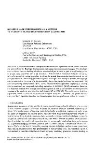
Two stage system for LV boundary estimation. Stage I (upper half, shown black in color) consists of three approaches: Pixel-classi cation approach, edge detection approach and the classi cation-edge fusion approach. Stage II (lower half, shown white in color), consists of the calibration stage which smoothes the raw boundaries produced in stage I. Left Half: O�-line training system, Right Half: On-line boundary estimation Right: The cross validation protocol consists of calibration parameters: N =377, K =188, L=187, F =2, P1 =100, P2 =100. Note the optimized points 20 are interpolated back to 100 points for polyline metric computation. Fig. 1.
The distance b ( 2 ) measuring the polyline distance from vertex boundary 2 is de ned by: ( ) b ( 2 ) = s 2 min sides B d
v; B
v
to the
B
d
v; B
2
(4)
d v; s
The distance vb ( 1 2 ) between the vertices of polylgon 1 and the sides of polygon 2 is de ned as the sum of the distances from the vertices of the polygon 1 to the closest side of 2 . X ( ) vb ( 1 2 ) = 2 d
B ;B
B
B
B
B
d
B ;B
v2 vertices B1
d v; B
On reversing the computation from 2 to 1 , we can similarly compute vb ( 2 1 ). Using Eq. 4, the polyline distance between polygons, s ( 1 : 2 ) is de ned by: vb ( 1 2 ) + vb ( 2 1 ) (5) s ( 1 : 2 ) = (# 2 +# 2 ) B
B
d
D
D
B
d
B
B ;B
B1
vertices
Using the above de nition, the overall mean can be given as: poly NFP
e
=
PFt PNn =1
=1
F
d
B
B ;B
B
B ;B
vertices
error epoly NFP
B2
of the calibration system
s (Gnt ; Cnt )
(6)
D
�
N
where, s ( nt nt ) is the polyline distance between the ground truth nt and calibrated polygons nt for patient study and frame number . D
G
;C
G
C
n
t
Linear vs. Quadratic Optimization Algorithms
5 Quadratic Vs. Linear Optimization Results
115
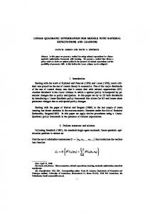
Suri et al. showed the linear calibration with convex information [5] [6] [7] [9] [10] for di�erent data sets (N ) ranging from 245 to 377. Using the cross validation protocol discussed in section 3, the polyline mean error in linear calibrator for InCM was 3.47 mm when N =291. Corresponding estimated boundaries are shown in g. 2. We here show results for the quadratic calibration under InCM conditions. The optimization curve for cross-validation is shown in g. 1 (right) with a dip when P =20. The corresponding mean error epoly NFP =2.49 mm. The calibration parameters were: N =377, F =2, K =188, P1 =100, P2 =100. The mean error when patient boundary lies both in training and testing data (TT case) condition is below 2 mm. The mean error for InCM technique under 4 conditions are: Without apex: 4.09 mm, with apex alone: 3.59 mm, with apex and AoV (linear): 2.97 mm, with apex and AoV (quadratic): 2.49 mm.
6 Diagnostic Clinical Acceptance and Discussions The mean error over ED and ES frames using a cross validation protocol and polyline distance metric was 2.49 mm over the database of 377 patient studies. The goal of the diagnostic system was 2.5 mm. InCM vs. IdCM: We also observed that when the training data was less (around 245 patient studies) then the IdCM technique was performing better than the InCM technique, and when the data was larger than 291 patient studies then the InCM technique was performing better than the IdCM technique. One reason of large error in IdCM with low data was due to the large number of coe�cients it had to compute. Also we used the singular value decomposition to evaluate the classi er matrix, Q, which is very critical in inverse computations, a full rank matrix in InCM was more superior to a full rank matrix in IdCM with large data size. Dynamics and Apparatus Design: Though we are able to obtain a goal on the cost of the heavy data processing, it may be worth while to discuss if computer processing of huge data is the only approach to handle the poor quality data sets (LVgrams). If careful analyzation is done, we nd that there can be less complexity in computer processing (LV classi cation, edge detection, calibration) if the LV chamber would receive enough contrast agent (dye). How can we improve the apparatus setup to inject dye in apical zone ? One way would be to bring a change in curvature of the catheter for handling variability of the LV's. If the LV is more longitudinal we should be able to change the curvature of the catheter to let dye ow towards the apex. On the contrary if the heart is very wide or huge, can a dual catheter facing opposite walls be a good choice ? One catheter can be used for lling the anterior side while the other catheter can be used to ll the inferior side. Another possibility would be to look over the lateral movement of the catheter during the motion of the LV . If we can detect the crests and troughs of the LV border muscles, we can then ll the apical zone using computer control. Careful design is feasible by controlling the
uid dynamics inside the LV chamber to improve the quality of the LVgrams.
116
J.S. Suri, R.M. Haralick, and F.H. Sheehan
7 Conclusions & Acknowledgements We compared the two training-based linear and quadratic calibration algorithms: the identical coe�cient and the independent coe�cient . We showed that the mean boundary error under quadratic calibration is better than the linear calibration with convex information of the LV. The mean error over end diastole and end systole frames using a cross validation protocol and polyline distance metric is 2.49 mm over the database of 377 patent studies. The goal of the diagnostic system is 2.5 mm. The software runs on PC and SUN work stations and written in C language. The authors thank Professors Linda G. Shapiro, Dean Lytle, Arun K. Somani, D. D. Meldrum, Werner Stuetzle, and Dr. Ajit Singh, Siemens for motivations.
References 1. Dumesnil et al.: LV Geometric Modeling and Quanti cation, Circulation (1979). 2. VanBree and Pope: Improving LV Border Recognition Using probability surfaces, IEEE Computers in Cardiology, pp. 121-124 (1989). 3. T.F. Cootes, C.J. Taylor, D.H. Cooper and J. Graham: Active Shape models: Their Training and Applications, Computer Vision and Image Understanding, Vol. 61, No. 1, January, pp. 38-59 (1995). 4. C. K. Lee: Ph.D Thesis, Department of Electrical Engineering, University of Washington, Seattle (1994). 5. Jasjit S. Suri, R. M. Haralick and F. H. Sheehan: Two Automatic Calibration Algorithms for Left Ventricle Boundary Estimation in X-ray Images, Proceedings of IEEE-Engineering in Medicine and Biology, Oct 31-Nov. 3 (1996). 6. Jasjit S. Suri, R. M. Haralick and F. H. Sheehan: Systematic Error Correction in automatically produced boundaries in Low Contrast Ventriculograms, International Conference in Pattern Recognition, Vienna, Austria, Vol. IV, Track D, pp. 361-365 (1996). 7. Jasjit S. Suri, R. M. Haralick and F. H. Sheehan: Accurate Left Ventricle Apex Position and Boundary Estimation From Noisy Ventriculograms, Proceedings of the IEEE Computers in Cardiology, Indianapolis, pp 257-260 (1996). 8. Jasjit S. Suri, R. M. Haralick and F. H. Sheehan: Left Ventricle Longitudinal Axis Fitting and LV Apex Estimation using a Robust Algorithm and its Performance: A Parametric Apex Model, International Conference in Image Processing, Santa Barbara, 1997, Volume III of III, IEEE ISBN Number 0-8186-8183-7, pp 118-121 (1997). 9. Jasjit S. Suri, R. M. Haralick and F. H. Sheehan: A General technique for automatic Left Ventricle Boundary Validation: Relation Between Cardioangiograms and Observed Boundary Errors, Journal of Digital Imaging, Vol. 10, No.2, Suppl 1, May, pp 1-7 (1997). 10. Jasjit S. Suri, R. M. Haralick and F. H. Sheehan: E�ect of Edge Detection, Pixel Classi cation, Classi cation-Edge Fusion Over LV Calibration, A two Stage Automatic system, 10th Scandinavian Conference on Image Analysis (SCIA '97), June 9-11, Finland (1997). 11. Jasjit S. Suri, R. M. Haralick and F. H. Sheehan: Two Automatic TrainingBased Forced Calibration Algorithms for Left Ventricle Boundary Estimation
Linear vs. Quadratic Optimization Algorithms
117
in Cardiac Images, Proceedings of IEEE-Engineering in Medicine and Biology, Chicago, Oct 31-Nov.2, ISBN 0-7803-4265-9(CD-ROM) SOE 9710002, pp. 528532 (1997). 12. Jasjit S. Suri, R. M. Haralick and F. H. Sheehan: Automatic Quadratic Calibration for Correction of Pixel Classi cation Boundaries to an Accuracy of 2.5 Millimeters: An Application in Cardiac Imaging, Proceedings of Int. Conference in Pattern Recognition, Brisbane, Austrialia, pp. 30-33, Aug. (1998).
Fig. 2. Upper (left & right): ED Input and output to the Quadratic Calibration System along with the ground truth boundary. Bottom: ES Input and output. Calibration Parameters: N =377, K =188, L=187, F =2, P1 =100, P2 =20, Mean error (epoly NFP ) = 2.49 mm.