ABSTRACT: The design and configuration of an effective supply chain has been ...... Brown G., Gerald, Harrison P. Terry, and Trafton L.,Linda, Global Supply.
OPTIMISATION BASED STRATEGIC CONFIGURATION OF DISTRIBUTION NETWORK
Xudong Xie, Arun Kumar, Robert De Souza Centre for Engineering and Technology Management School of Mechanical & Production Engineering Nanyang Technological University Nanyang Avenue, Singapore 639798
ABSTRACT: The design and configuration of an effective supply chain has been widely recognised
as being of fundamental importance to the business performance of all companies within the present competitive market. In supply chain structure, outbound physical distribution channel can be regarded as the key stage which will meet the customers’ demand and requirements directly. This paper mainly involves strategic configuration of distribution network by using mathematical optimisation method. The objective of this study is to obtain an optimal strategic scheme of distribution network which can meet customer demand with minimum operating cost and time. Especially within the electronics manufacturing in Asia-Pacific, application of postponement concept leads to importance of Bill of Distribution (BOD) in distribution processes. The model in this paper will consider the constraints of these special requirements. Finally, this optimisation model is applied to design the distribution network structure of a computer manufacturing company.
INTRODUCTION In today’s competitive business environment industry has recognised the importance of efficient supply chain management. Due to the recent trends in international procurements, new information technologies, increasing pressure from customers on responsiveness and reliability and the globalisation of operations and markets, supply chain management has become a challenge and an opportunity. Ganeshan [1999] addressed the supply chain management as follows: A supply chain is a network of facilities and distribution options that performs the functions of procurement of materials, transformation of these materials into intermediate and finished products, and the distribution of these finished products to customers. A typical supply chain structure is shown in Figure 1. Supply chain includes its upstream supplier network and its downstream distribution channel. As a final part of supply chain, the distribution channel is always regarded as the segment to face the final customers directly. Therefore, the management of distribution channel also becomes more critical [Cohen and Lee, 1988]. A firm’s external downstream/outbound supply chain as illustrated in Figure 1 encompasses all the downstream distribution channels, processes, and functions that the product passes through on its way from the product source---plants to the end customer. For example, an automotive company’s distribution network includes its finished goods and pipeline inventory, warehouses, dealer network, and sales operations. This particular distribution channel is relatively short. Other types of supply
1
chains may have relatively small internal supply chains but fairly long downstream distribution channels [Handfield, 1996]. Outbound(distribution channel)
Inbound (Procurement channel)
Mfg.
Supplier
Distribution Center Supplier
Supplier
Materials HUB
Mfg.
DC
Mfg.
Region DC
Customer
Region DC
Customer
Region DC
Customer
Materials Flow Information and cash flow
Figure 1. Typical supply chain structure It is significant for companies to build an optimal structure of distribution channel with high performance. Especially for strategic configuration, it is impossible that companies change their location of distribution centre, region depots or links between individual facilities very often. Therefore, designing strategic structure of distribution network optimally plays more and more important role in decision-making processes of companies.
APPROACHES AND DECISIONS TO DESIGN DISTRIBUTION NETWORK The area of mathematical optimisation is well developed and a widely diversified range of tools is available for the management scientist [Mourits and Evers, 1996]. Until now, management science has been involved in improving the power of the mathematical tools with good results. Numerous distribution models have been developed for multiple objective facility location decisions [Aikens, 1985], transshipment centre location problems [Bhaskaran, 1992] and multi-period network flow problems [Glover, et al, 1992]. The earliest work in this area, although the term “supply chain” was not in vogue, was by Geoffrion and Graves [1974]. They introduce a multi-commodity logistics network design model for optimising annualised finished product flows from plants to distribution centre (DC), and to the final customer. Georffrion and Powers [1993] later give a review of the evolution of distribution strategies over the past twenty years. Cohen and Lee [1985] have developed a conceptual framework for manufacturing strategy analysis, where they describe a series of stochastic sub-models, that considers annualised product flows from raw material vendors via intermediate plants and distribution echelons to the final customers. Min and Eom [1994] present a decision support system for global logistics in which they propose and design the conceptual framework of an integrated DSS linked by worldwide communication and distribution networks. Arntzen et al, [1995] provide the most comprehensive deterministic model for supply chain management. In their paper, the objective function is to minimise a combination of cost and time elements. Unique to this model was the explicit consideration for duty and their recovery as the product flowed through different countries. The decision support systems mentioned above focus on location-allocation problems in networks consisting of three or more echelons of participants: plants, warehouses and customers. The primary objective in these papersis to determine: The number, location and size of distribution centres to open,
2
The number, location and size of regional depots to open, The links between different facilities, Which customer zones they should be assigned to serve, The flows of goods throughout the system. Additionally, the distribution processes of the electronics manufacturing industry are utilising new concepts and ideas. A typical distribution concept is introduced in the following sections.
CHARACTERISTICS IN DISTRIBUTION CHANNEL
Postponement in distribution Besides understanding the flow of products through the supply channel, various enterprises must also find answers to questions: what should be the stocking state of their inventories? At what stage in the flow process should inventory be in its finished state? Delaying final labelling, assembly, or packaging (localisation) until the last moment is known as the principle of postponement. The objective of this principle is to minimise the risk of carrying finished forms of inventory at various echelons in the channel by delaying product differentiation to the latest possible moment before customer purchases [David, 1996]. The use of inventory postponement is critical for distributors because it basically reduces the cost of carrying inventory and optimises on logistics resources, such as transportation and warehousing. The only caveat to effective use of inventory postponement is the existence of efficient processes that facilitate the creation of the final product and timely delivery to the customer [Lee, 1996]. Bill of Distribution Due to extensive use of postponement principle in electronics manufacturing, the Bill of Distribution (BOD) will become more complicated and different from the previous version, and the Bill of Materials (BOM). It is known that the Bill of Materials is a kind of list file that describes the structural relationship of product to be assembled in manufacturing [Vollmann, et al, 1984]. BOM should include all subassembly components, parts, raw materials and their quantities. BOM is the master file to run the MRP system. Therefore, the structural and assembling relationship between different parts and components will be represented in BOM. Afterwards, we can find some differences in these two similar concepts---BOM and BOD. It is obvious that the operation of inbound supply chain and manufacturing must depend on BOM. Bill of Distribution (BOD) is the key data file in the application of distribution resource planning (DRP) [David, 1996]. BOD links supplying and satellite warehouses together, similar to the way the BOM links components items to their assembly parents. Although BOD utilises the concept and structure of the manufacturing BOM, it mainly identifies the supplying and assembling point relationship between the candidate suppliers in distribution procedure. Especially in application of postponement principle in distribution, the BOD seems to be more effective to express this relationship. After the development of the principle of postponement and the Bill of Distribution, the optimisation model has been considering the necessary constraints from the special structural requirements in designing the distribution channel networks.
3
OPTIMISATION MODEL FOR DESIGN OF DISTRIBUTION NETWORK Overall requirements The optimisation model in this report focuses mainly on location-allocation problems, strategic capacity configuration, and strategic transportation configuration. The primary objective of this optimisation model is to determine: The number, location, and size of alternative plants to open The number, location, and size of alternative distribution centres to open The number, location, and size of alternative regional depots to open The link between different nodes in distribution chain The transportation mode selection The shipment size in different transportation modes The rough capacity requirements on individual plants, depots, and transportation modes Additionally, this model uses several sets of double-subscripted variables as opposed to a single set triple or four-subscripted variables to represent the link indicator variables and shipment quantities variable. This approach leads to a significant reduction in the number of variables used in the model. For instance, for a design problem with 5 alternative manufacturers, 5 alternative distributors, and 20 retailers, the number of variables required by the proposed model is equal to 125=(5)(5)+(5)(20), compared to 500=(5)(5)(20) variables in a traditional distribution model using triple-subscripted variables. In four subscripted variables, for example, 5 alternative manufacturers, 5 alternative distribution centres, 10 regional distribution depots, 30 customer zones, the number of variables is equal to 7,500=(5)(5)(10)(30), and the number of variables in this model is equal to 375=(5)(5)+(5)(10)+(10)(30). This approach is used by Tyagi and Das [1995].
Literal description of the mathematical model
Decision Variables The identified variables for selecting the links among the four structures proposed, The identified variables for selection of alternative manufacturers, The identified variables for selection of transportation modes, The identified variables for opening in alternative distribution centres, The identified variables for opening in alternative regional distribution depots (RDD), Procurement quantities from the manufacturers or supply sources, Shipment quantities in different transportation modes (this includes the truck, the railway, the air, and the sea), Inventory quantities in the various storage points (DCs, RDDs, and so on). Objective function Minimise total cost =λ*(Production fixed costs +Production variable costs + Transportation fixed cost + Transportation variable cost + Warehouse fixed cost + Warehouse variable cost)+(1λ)*(Production lead-time + Shipping time) Where, λ is weight factor, 0≤λ≤1, used for convex linear combination of cost and activity time. Constraints System constraints 4
• • • • • • •
Available quantities supplied from manufacturers, Minimum and maximum warehouse capacities constraints, Minimum and maximum manufacturer’s capacities constraints, Minimum and maximum transportation capacities constraints, Customers’ demand, Inbound and outbound balance for distribution centre warehouse, Inbound and outbound balance for regional distribution centre warehouse.
User-specified Constraints: • Specifically include or exclude a manufacturer, • Specifically include or exclude a distribution centre, • Specifically include or exclude a regional distribution depots, • Use a specified link between different nodes in distribution network, • Use any single warehouse to make shipments to a regional retailer, • Use a given set of warehouses to make shipments to the customers, • Use a given set of manufacturers to make shipment to a warehouse. These constraints will lead the network structure to meeting the requirement of postponement and Bill of Distribution. Model constraints: • Customer demand is met for each product, in each customer region, • Production and inventory volumes are accounted for, • Products are manufactured using component recipes (it is the constraints from the Bill of distribution and postponement). Here, this model stresses the structural constraints from the Bill of Distribution and postponement concepts. The structural constraints indicate that the components for final assembling and differentiation should be available at the suitable place and time. Most of the sub-assembling tasks will be completed at the distribution centre, and some of the final assembling tasks are arranged at regional depot. Therefore, the number of components with proportional relationship must be transferred from the individual suppliers. For instance, one final printer’s assembling needs one set of header driver board, two sets of plastic gears, one set of key pad board. The number of these parts transferred from individual suppliers should satisfy this proportional relationship in product structure. The formulated optimisation model is exhibited in the Appendix.
EXPERIMENTAL SOLUTION XYZ Company is the manufacturer of Personal Computer‘s main component, whose products include packaging, plastic parts, keyboard, PCBA of computers. Most of its plants and suppliers, that produce these parts and components, are located in different regions in Asia. Moreover, the company can receive supplies from alternative plants and suppliers. The problem is that the company must decide to choose the optimal physical configuration of the distribution channel. For example, there are three alternative plants producing HDDA and located in Malaysia, Taiwan, and Singapore respectively. Similar situation exists in the selection of other parts, the sub-assembling location, and the final assembling location. The problem is to select the alternatives. This company needs to decide its distribution network with the minimum operating cost and activity time. The model presented in this paper is able to determine the plant manufacturing specific product, alternative site for building the distribution centre, site to open the regional distribution 5
depot for the processes of final testing and assembling tasks, and capacity configuration of plants. Further, the selection of transportation modes is also the main concern.
Optimal scheme
Figure 2. The Simulation results on total operating cost
Optimal Scheme
Figure 3. Simulation results on total activity time As described in the previous section and Appendix, we have established an optimisation model, which has been used to solve this type of problem. Although the integer programming application can result into complex problem, it can solve the resource allocation ideally. Moreover, the number of variables in the model has been reduced by using several sets of double-subscripted variables as opposed to a single set, triple or four-subscripted variables to represent the link indicator variables, and shipment quantities variables. The optimal scheme has been obtained in less than five minute of computing time by LINDO software on PC (PII 350M, 64M RAM). In order to validate the optimisation model, a simulation model is developed. By adjusting the individual parameters, the different results can be obtained. These adjustments include those on transportation model, links between facilities, the production and shipping sizes, and inventory level stored at distribution centre and regional depot, and so on. Figures 3 and 4 show the results from the simulation model. 6
Figure 2 shows the simulation results on total cost based on numerous network configurations. The red curve is the result of optimal scheme calculated by the proposed model. The others are nonoptimal schemes. This result assists us to validate the optimisation model and optimal scheme. Figure 3 displays the simulation results on activity time. It is observed that the total activity time in optimal scheme is not the minimal one. The weight factor λ leads to this situation. It implies that more attention should be paid to the total operating cost than the total activity time in the optimisation model of this paper. Thus, λ can be used to balance the weight between these two objective variables. The simulation results prove the statement that an optimal solution for configuration of distribution network can be obtained.
CONCLUSION This paper firstly introduces the definition of supply chain management and the related literature. In electronics industry, the application of the principle of postponement leads to the development of Bill of Distribution (BOD). Consequently, the optimisation model for the design of distribution channel has to consider these constraints which guarantee the distribution channel to meet the structural requirements of the Bill of Distribution. A mathematical programming model has been developed in this study. The model complements a physical design of distribution network at strategic level. Although this model is not perfect yet, a strategic and brief optimisation solution is feasible. The model has two features: double subscripted variables decrease the number of variables, and the other is to form constraints to satisfy the requirement of Bill of Distribution‘s structure of products. By using this optimisation model, a computer manufacturing company successfully completed its design of distribution network with minimal operating cost and activity time. This approach is very effective and can be used as an important tool in the decision making process of supply chain.
Appendix I. Indices m = the number of alternative plants, or suppliers, n = the number of alternative distribution centres, d = the number of the regional depots or regional distribution centres, c = the number of the customer zones, p = the number of the product types, q = the number of the transportation modes, such as sea, railway, truck and air etc. i = {1,2,…m}, j = {1,2,…n}, k = {1,2,…d}, l = {1,2,…c}, r = {1,2,…q}, g = {1,2…p}, o: the original site of product flow t: The destination site of product flow
7
II. Decision Variables:
vmig : Binary integer variable; 1 if ith candidate manufacturer to produce gth product is operational; otherwise 0, vx jg : Binary integer variable; 1 if jth candidate distribution centre to store gth product is operational; otherwise 0,
vykg : Binary integer variable; 1 if kth candidate regional depot to store gth product is operational; otherwise 0,
vlotgr : Binary integer variable; 1 if the link from original site to destination site that transport gth product by mode r is operational,
vs otgr : the amount of the products shipped from original site to destination site, ( units) ,
vpog : the storage amount of the gth product on the certain site o , ( units ), III. Parameters: CFIXLog : the annual fixed cost of storing gth product on the certain site o, $/year*unit, CFIXS otgr : the annual fixed cost on the link from the original site to the destination site that transports gth product by shipping mode r, $/year*unit*mode, CPMAX ig : the maximum capacity of producing the gth product on the i th manufacturer, units, CPMIN ig : the minimum capacity of producing the gth product on the i th manufacturer, units, CUNIT fg : the unit cost for processing (producing or storing) the gth product on fth site, $/unit*product; f belongs to one of m,n,d, CSHIPotgr : the unit cost for shipment from original site to destination site that transports ith product by mode r, $/unit*product*mode, DMNDlg : the demand of the gth product on the l th customer zone, units, CSMAX gr :the maximum capacity of the gth product shipped by the r th shipping mode, units, CSMIN gr :the minimum capacity of the gth product shipped by the r th shipping mode, units, PDAYog : The process time of the gth product at the oth site, TDAYotgr : The shipping time of the gth product by the rth shipping mode from the original site to the destination site,
IV. Decision Function Min
8
d c m p q n ∑ ∑ ∑ ∑ vs ijgr * CSHIP ijgr + ∑ vs ikgr * CSHIP ikgr + ∑ vs i lg r * CSHIP i lg r + k l i g r j n p q p q d c d c + + vs * CSHIP vs * CSHIP vs * CSHIP jkgr j lg r k lg r ∑g ∑r ∑k jkgr ∑l j lg r ∑k ∑g ∑r ∑l k lg r ∑ j d c m p q n ∑ ∑ ∑ ∑ vl ijgr * CFIXS ijgr + ∑ vl ikgr * CFIXS ikgr + ∑ vl i lg r * CFIXS i lg r + k l λ + i g r j p q p q n d c d c ∑ ∑ ∑ ∑ vl jkgr * CFIXS jkgr + ∑ vl j lg r * CFIXS j lg r + ∑ ∑ ∑ ∑ vl k lg r * CFIXS k lg r l k g r l j g r k p p p m p m n d + ∑ ∑ vm ig ∗ CFIXL ig + ∑ ∑ vx jg ∗ CFIXL jg + ∑ ∑ vy kg ∗ CFIXL kg + ∑ ∑ vp ig * CUNIT ig i g j g k g i g n p p d + vp jg * CUNIT jg + ∑ ∑ vp kg * CUNIT kg ∑ ∑ j g k g
∑ PDAY ig * vp ig + ∑ PDAY jg * vp jg + ∑ PDAY kg * vp kg j, g k,g i , g p q d c m n + (1 − λ ) ∑ ∑ ∑ ∑ vs ijgr * TDAY ijgr + ∑ vs ikgr * TDAY ikgr + ∑ vs i lg r * TDAY i lg r + i g r j k l + c n p q d d p q c ∑ ∑ ∑ ∑ vs jkgr * TDAY jkgr + ∑ vs j lg r * TDAY j lg r + ∑ ∑ ∑ ∑ vs k lg r * TDAY k lg r l k g r l j g r k
V. Constraints: A. The customer demand: 1).
d
q
k
r
∑∑ vs
k lg r
= DMNDlg
∀ l,g
B. The Inbound and outbound balance for distribution centre warehouse, regional depots; d
q
n
q
k
r
j
r
d
q
k
r
(2a). vp jg + ∑∑ vs jkgr ≤ ∑∑ vsijgr ≤ vpig
∀ i,g
(2b). vp kg + ∑∑ vs k lg r ≤ ∑∑ vs jkgr ≤ vp jg (2c).
c
q
l
r
∑∑ vs
k lg r
∀ j,g
≤ vp kg
∀ k,g
C. The Manufacturers’ capacity, warehouses’ capacity: (3a). vmig * CPMIN ig ≤ vp ig ≤ vmig * CPMAX ig
∀ i,g
(3b). vx jg * CPMIN jg ≤ vp jg ≤ vx jg * CPMAX jg
∀ j,g
(3c). vy kg * CPMIN kg ≤ vp kg ≤ vy kg * CPMAX kg D. The transportation model ‘s capacity From manufacturer: (4a-1). vlijgr * CSMIN gr ≤ vsijgr ≤ vlijgr * CSMIN gr
∀ k,g
(4a-2). vlikgr * CSMIN gr ≤ vsikgr ≤ vl kjgr * CSMIN gr
∀ i,k,g,r
(4a-3). vli lg r * CSMIN gr ≤ vsi lg r ≤ vli lg r * CSMIN gr From distribution center: (4b-1). vl jkgr * CSMIN gr ≤ vs jkgr ≤ vl jkgr * CSMIN gr
∀ i,l,g,r
∀ i,j,g,r
9
∀ j,k,g,r
(4b-2). vl j lg r * CSMIN gr ≤ vs j lg r ≤ vl j lg r * CSMIN gr
∀ j,l,g,r
From regional depots: (4c). vl k lg r * CSMIN gr ≤ vs k lg r ≤ vl k lg r * CSMIN gr
∀ k,l,g,r
E. The location and number limit of distribution centre: n
(5a).
∑ vx
jg
=1
∀g
jg
≤p
∀j
j
p
(5b).
∑ vx g
F. The location and number limit of regional depots: p
(6).
∑ vy
kg
∀k
≤ c−C
g
G. The location and number limit of manufacturers: p
(7).
∑ vm
ig
∀i
≤ m−M
g
H. The network flow logic limit: (8a). vlijgr ≤ vmig
∀ i,j,g,r
(8b). vlikgr ≤ vmig
∀ i,k,g,r
(8c). vli lg r ≤ vmig
∀ i,l,g,r
(9a). vlijgr ≤ vx jg
∀ i,j,g,r
9b). vl jkgr ≤ vx jg
∀ j,k,g,r
(9c). vl j lg r ≤ vx jg
∀ j,l,g,r
(10a). vlikgr ≤ vy kg
∀ i,k,g,r
(10b). vl jkgr ≤ vy kg
∀ j,k,g,r
(10c). vl k lg r ≤ vy kg I. The Bill of Distribution and postponement requirement: (11a-1). vl i1 jg1r = vl i 2 jg 2 r = vl i 3 jg 3r = ... = vl imjgmr = 1
∀ k,l,g,r
(11a-2). α 1 * vs i1 jg1r = α 2 * vsi 2 jg 2r = α 3 * vsi 3 jg 3r = ... = α m * vsimjgmr
∀ i,j,g,r
(11b-1). vl j1 jg1r = vl j 2kg 2 r = vl j 3kg 3r = ... = vl jmkgmr = 1
∀ j,k,g,r
(11b-2). β 1 * vs j1 jg1r = β 2 * vs j 2 kg 2r = β 3 * vs j 3kg 3r = ... = β m * vs jmkgmr J. Generic system constraints: All variables >= 0, vmig , vx jg , vy kg , vlijgr are binary integer variables, 0 or 1;
∀ j,k,g,r
∀ i,j,g,r
α 1 , α 2 ,..., and , β 1 , β 2, ... are the structural coefficient in Bill of Distribution. λ is objective weight factor, 0≤λ≤1, used for convex linear combination of cost and weighted activity time, C,M are the number specified by designer.
10
References Aikens, C. H., Facility Location Models for Distribution Planning, European Journal of Operational Research, Vol. 22, 1985, pp.263-279 Arntzen, B.C., Brown G., Gerald, Harrison P. Terry, and Trafton L.,Linda, Global Supply Chain Management at Digital Equipment Corporation. Inerfaces, Jan-Feb, 1995 Bhaskaran, S., Identification of Transshipment Centre Locations, European Journal of Operation Research, Vol. 63, 1992, pp.141-150 Das Chandrasekhar and Tyagi Rajesh, Wholesaler: A Decision Support System for Wholesale Procurement and Distribution, International Journal of Physical Distribution & Logistics Management, Vol.24, No.10, pp.4-12, 1994 Cohen, M. A. and Lee H. L., Manufacturing Strategy Concepts and Methods, in Kleindorfer, P. R. Ed., The Management of Productivity and Technology in Manufacturing, pp.153-188, 1988 Cohen, M. A. and Lee H. L., Strategic Analysis of Integrated Production-Distribution Systems: Models and Methods. Operations Research, 36, 2, 216-228, 1988 David Frederick Ross, Distribution Planning and Control, New York: Chapman & Hall, 1996 Ganeshan Ram, An Introduction to Supply Chain Management, Http://silmaril.smel.psu.edu/misc/supply_chain_intro.html, 1999 Geoffrion, A., and Graves G., Multicommondity Distribution System Design by Benders Decomposition. Management Science, Vol. 29, No. 5, 1974, pp. 822-844 Geoffrion, A. and Powers R., 20 Years of Strategic Distribution System Design: An Evolutionary Perspective, Interfaces, 1993 Glover, F., Klingman, D., and Philips, N. V., Network Models in Optimisation and their Applications in Practice, Wiley-Interscience, New York, NY, 1992 Handfield Robert B., Introduction to Supply Chain Management, New Jersey: Prentice Hall, 1996 Lee. H. L., Effective Inventory and Service Management Through Product and Process Design, Operation Research, Vol.44, No. 1, pp.151-159, 1996 Min Hokey and Eom Sean B., An Integrated Decision Support System for Global Logistics, International Journal of Physical Distribution & Logistics Management, Vol. 24, No. 1, pp.29-39, 1994 Lee Hau L., Effective Inventory and Service Management through Product and Process Redesign, Operation Research, Vol. 44, No. 1, 1996 Mourits Marcel and Evers Joseph J. M., Distribution Network Design: An Integrated Planning Support Framework, Logistics Information Management, Vol. 9, No. 1, pp.45-54, 1996 Tyagi, Rajesh and Das Chandrasekhar, Manufacturer and Warehouse Selection for Stable Relationship in Dynamic Wholesaling and Location Problems, International Journal of Physical Distribution & Logistics management, Vol. 25, No.6, 1995, pp.54-72 Vollmann Thomas E. and Berry William L and Whybark D. Clay, Manufacturing Planning and Control System, IRWIN. USA, 1984
11