Dec 9, 1997 - Computational Mechanics, 23 (1999) 117â123. 1 ... Aerospace Engineering and Mechanics ... The computations are based on the Deformable- ..... in this paper, we use perfect slip condition on the surface-piercing body.
1
Computational Mechanics, 23 (1999) 117–123
Parallel finite element computation of free-surface flows I. G¨ uler, M. Behr and T. Tezduyar Aerospace Engineering and Mechanics Army HPC Research Center University of Minnesota 1100 Washington Avenue South Minneapolis, MN 55415, USA December 9, 1997 revised January 28, 1998 Abstract In this paper we present parallel 2D and 3D finite element computation of unsteady, incompressible free-surface flows. The computations are based on the DeformableSpatial-Domain/Stabilized Space-Time (DSD/SST) finite element formulation, which takes automatically into account the motion of the free surface. The free-surface height is governed by a kinematic free-surface condition, which is also solved with a stabilized formulation. The meshes consist of triangles in 2D and triangular-based prism elements in 3D. The mesh update is achieved with general or special-purpose mesh moving schemes. As examples, 2D flow past spillway of a dam and 3D flow past a surfacepiercing circular cylinder are presented.
1. Introduction Free-surface flow problems involve spatial domains which change their shapes due to the motion of the free surface. The location of the free surface is not known a priori and is determined as part of the overall solution. This leads to a geometric nonlinearity in addition to the nonlinearities that are already part of the Navier-Stokes equations. The Deformable-Spatial-Domain/Stabilized Space-Time (DSD/SST) finite element formulation was first introduced in Tezduyar et al. (1992a) and Tezduyar et al. (1992b), and was applied to many classes of flow problems involving moving boundaries and interfaces (see e.g. Tezduyar et al. (1996)). In this approach, the stabilized finite element formulations of the governing equations are written over the space-time domain of the problem. With this, changes in the shape of the spatial domain due to the motion of the boundaries and interfaces are taken into account automatically. This approach gives us the capability to solve a large class of problems, such as free surfaces, two-fluid interfaces and fluid-structure interactions. The standard Galerkin formulation of incompressible flows can involve two well-known numerical instabilities. The first one is due to the presence of advection terms in the governing equations. The second numerical instability is unique to mixed methods and is caused by using unacceptable combinations of interpolation functions to represent the velocity and
2
Computational Mechanics, 23 (1999) 117–123
pressure fields. In the work reported here, the DSD/SST formulation is based on stabilization of the method with the Galerkin/least-squares approach. The finite element functions are linear both in space and time, continuous in space, but discontinuous in time. This discontinuity in time allows the computations to be carried out one space-time ”slab” at a time, where the ”slab” is a slice of the space-time domain between two consecutive time levels. It also gives us the option of changing the spatial discretization from one time step to another. In the DSD/SST formulation, a large, coupled system of nonlinear equations needs to be solved at every time step of the simulation. These systems are solved with Newton-Raphson iterations. Each step of the Newton-Raphson sequence requires the solution of a linear equation system. These systems are also solved iteratively, using the GMRES technique (Saad and Schultz (1986)). In Section 2, we review the Navier-Stokes equations of incompressible flows and describe the turbulence model. The stabilized finite element formulations are presented in Section 3. The mesh update method is discussed in Section 4. The issues concerning moving contact line and outflow boundary condition are addressed in Section 5 and Section 6, respectively. The elements used, especially the triangular-based prisms, are discussed in Section 7. In Section 8, we report simulation of 2D flow past spillway of a dam and 3D flow past a surfacepiercing circular cylinder. We provide our concluding remarks in Section 9. 2. Governing equations The computations are based on solution of the time-dependent Navier-Stokes equations of incompressible flows. We consider a viscous, incompressible fluid occupying at an instant t ∈ (0, T ) a bounded region Ωt ⊂ Rnsd , with boundary Γt , where nsd is the number of space dimensions. In the DSD/SST formulation, the spatial domain may change with respect to time, and the subscript t indicates such time-dependence. The symbols u(x, t) and p(x, t) represent the velocity and pressure. The external forces (e.g., the gravity) are represented by f(x, t). The momentum and mass balance equations can be written as follows: � � ∂u ρ + u · ∇u − f − ∇ · σ = 0 on Ωt ∀t ∈ (0, T ), (1) ∂t ∇·u =0 on Ωt ∀t ∈ (0, T ), (2) where the density ρ is assumed to be constant. The stress tensor σ can be decomposed into its isotropic and deviatoric parts: σ(u, p) = −pI + T.
(3)
We consider only the Newtonian fluids, for which the deviatoric stress is related linearly to the strain rate tensor: T = 2µε(u),
ε(u) =
� 1 ∇u + (∇u)T , 2
(4)
3
Computational Mechanics, 23 (1999) 117–123
where µ is the dynamic viscosity. The Dirichlet and Neumann-type boundary conditions are represented as u =g n·σ =h
on (Γt )g , on (Γt )h ,
(5) (6)
where (Γt )g and (Γt )h are complementary subsets of the boundary Γt . Boundary conditions imposed on the free surface consist of kinematic and dynamic conditions. The kinematic condition requires that the free surface is a material surface; i.e. the fluid particles which are at some time on the free surface always stay on it. This condition is used to describe the motion of the free surface. For a 3D problem, on the free-surface z = H(x, y, t), ∂H ∂H ∂H + us + vs − ws = 0 on S ∂t ∂x ∂y
∀t ∈ (0, T ),
(7)
where H is the free-surface elevation and the subscript s refers to quantities at the free surface. The domain S is the lower-dimensional region over which H is determined, typically obtained from Ωt by projection. The surface tension effects are neglected, and the stress-free condition is imposed as the dynamic condition on the free surface. The initial condition consists of a divergence-free velocity field specified over the entire domain: u(x, 0) = u0 ,
∇ · u0 = 0 on Ω0 .
(8)
In the present study, there are two dimensionless parameters that characterize the flow. They are the Reynolds number: Re =
ρUL , µ
(9)
which is the ratio of inertial forces to viscous forces; and the Froude number: U Fr = √ , gL
(10)
which is the ratio of inertial forces to gravity forces. In these definitions, U and L denote characteristic velocity and length, respectively. Because the typical meshes are not able to resolve the flow features well enough to fully capture turbulence effects at high Reynolds numbers, introduction of a turbulence model becomes necessary. In the present study, a simple Smagorinsky turbulence model is employed. In this model, the kinematic viscosity ν is augmented by an eddy viscosity νt which is defined as 1
νt = (Ch)2 (2ε(u) : ε(u)) 2 ,
(11)
where C is a constant and h is the element length defined here as the maximum of the edge lengths for the element. Here, we set C to 0.15.
4
Computational Mechanics, 23 (1999) 117–123
3. Stabilized finite element formulations The computations are based on the space-time finite element method, in which the weak form of the governing equations is written over the associated space-time domain of the problem. To construct the finite element function spaces for the space-time method we partition the time interval (0, T ) into subintervals In = (tn , tn+1 ), where tn and tn+1 belong to an ordered series of time levels 0 = t0 < t1 < · · · < tN = T . Let Ωn = Ωtn and Γn = Γtn . We will define the space-time slab Qn as the domain enclosed by the surfaces Ωn , Ωn+1 , and Pn , where Pn is the surface described by the boundary Γt as t traverses In . As it is the case with Γt , surface Pn is decomposed into (Pn )g and (Pn )h with respect to the type of boundary condition (Dirichlet and Neumann) being applied. For each space-time slab Qn , we define the following finite-dimensional trial solution ((Suh )n and (Sph )n ) and test function ((Vuh )n and (Vph )n ) spaces for the velocity and pressure: � � �nsd h . h (Suh )n = uh | uh ∈ H 1h (Qn ) ,u = g on (Pn )g , (12) � h � 1h �nsd h h h . (Vu )n = w | w ∈ H (Qn ) , w = 0 on (Pn )g , (13) � (14) (Sph )n = (Vph )n = ph | ph ∈ H 1h (Qn ) , where H 1h (Qn ) represents the finite-dimensional function space constructed over the spacetime slab Qn by using first-order polynomials in space and in time. The interpolation function spaces are discontinuous in time and continuous in space. The stabilized space-time formulation of Equations (1) and (2) can then be written h h h h h h as follows: given (uh )− n , find u ∈ (Su )n and p ∈ (Sp )n such that ∀w ∈ (Vu )n and ∀q h ∈ (Vph )n : � h � Z Z ∂u h h h + u · ∇u − f dQ + w ·ρ ε(wh ) : σ(uh , ph )dQ ∂t Qn Qn Z Z � h + h − + q h ∇ · uh dQ + (wh )+ n · ρ (u )n − (u )n dΩ Qn
Ωn
� � � � 1 ∂wh h h h h + u · ∇w − ∇ · σ(w , q ) + τMOM ρ ρ ∂t Qen e=1 � � � � h ∂u h h h h · ρ + u · ∇u − f − ∇ · σ(u , p ) dQ ∂t Z (nel )n Z X h h + τCONT ∇ · w ρ∇ · u dQ = wh · h h dP. (nel )n Z
X
e=1
Qen
(15)
(Pn )h
The following notation is being used in Equation (15): (uh )± n = lim u(tn ± ε), ε→0 Z Z Z . . . dQ = . . . dΩdt, Z
Qn
In
Ωh t
In
Γh t
Z Z . . . dP =
Pn
. . . dΓdt.
(16) (17) (18)
5
Computational Mechanics, 23 (1999) 117–123
The definitions of the stabilization parameters τMOM and τCONT can be found in Behr and Tezduyar (1994). The solution to Equation (15) is obtained for all of the space-time slabs Q0, Q1, . . . , QN −1 sequentially, and the computations start with h (uh )− 0 = u0 .
(19)
The stabilized finite-element formulation of Equation (7) can be written as �
� � h � nel Z h h X ∂H h ∂ψ ∂H h ∂ψ h ∂H h h ∂H h ∂H h dS ψ τDC + us + vs − ws dS + + ∂t ∂x ∂y ∂x ∂x ∂y ∂y e S S e=1 � � � � nel Z h h h h X ∂H h h ∂ψ h ∂ψ h ∂H h ∂H h + τSUPG us + vs + us + vs − ws dS = 0. (20) ∂x ∂y ∂t ∂x ∂y e e=1 S
Z
h
The stabilization parameter for the discontinuity-capturing term can be defined as τDC = Ch2s r(H h ), ∂H h ∂H h ∂H h + u + v − w ∂t s ∂x s ∂y s r(H) = , max H − min H
(21) (22)
or, alternatively, as τDC = CUhs ,
(23)
where C is typically set to 1. The U in Equation (23) represents reference velocity. The “artificial diffusion” form of the coefficient (23) is intended to be used only as a transitional measure, allowing the simulation to continue through dramatic surface deformations encountered during the initial stages. As the free surface stabilizes, more accurate transient behavior can be obtained using the consistent form (21). The stabilization parameter for the SUPG term has the standard form: τSUPG =
hs , 2 |us |
(24)
where hs is a measure of the element length. Both of the nonlinear systems given by Equations (15) and (20) are solved with the Newton-Raphson method. The solution of flow variables and free surface updates are carried out in succession within the nonlinear iteration. This formulation has been implemented on parallel architectures, under data parallel model using Connection Machine Fortran Kennedy et al. (1994), and under message passing model using MPI library Tezduyar et al. (1996). 4. Mesh update method In computation of free-surface flows with an interface-tracking technique, one needs to handle the changing spatial domain by updating the mesh. Two main update approaches can be
Computational Mechanics, 23 (1999) 117–123
6
employed for this purpose. The first one is based on moving the nodal points of the mesh. The second one is based on remeshing (i.e. generating a new set of nodes and elements). These two approaches can be used alone or in combination. The motion of the nodal points will be subject to boundary conditions conforming to the motion of the free surface. The motion of the free-surface is determined at every nonlinear iteration by solving the equation governing the free-surface height. Once the new location of the free surface is known, we can use two different methods to determine the motion of the nodal points. One approach is to employ an automatic mesh moving scheme (Johnson and Tezduyar (1994)). In this method, the modified equations of linear elasticity are solved using the finite element method to determine the internal nodal displacements. We can combine automatic mesh moving with remeshing as needed. Generation of the starting mesh and remeshing are typically accomplished by using an automatic mesh generator. The automatic mesh moving technique is used in the 2D example presented later in this paper. Another approach is to use a special-purpose mesh moving scheme, typically in conjunction with a special-purpose mesh generator, to specify the motion of the mesh based on some pre-defined rules. This approach can be employed only in cases where the changes in the shape of the spatial domain is sufficiently simple. An earlier example, parallel 3D computation of sloshing in a vertically vibrating container, can be found in Behr and Tezduyar (1994). In the 3D free-surface flow problem presented in Section 8.2, we move the nodal points only in the vertical direction. Once the new location of the free surface is calculated, the nodes are redistributed along the vertical lines according to a geometric progression rule. By doing so, we place the smaller elements near the free surface. An advantage of this method over the automatic mesh moving scheme is that we don’t need to solve an additional equation system to update the mesh at every nonlinear iteration. 5. Moving contact line In computation of free-surface flow past a solid object, special attention needs to be paid to handling a contact line where the free surface intersects the solid boundary. Imposing no-slip condition at the contact line gives rise to a stress singularity there. To circumvent this problem, the no-slip condition needs to be relaxed. This can be achieved by employing Navier’s slip condition Navier (1823) that makes the tangential components of stress at the solid surface proportional to the local slip velocity: 1 (I − nn) · (n · σ) = − (I − nn) · (u − v) , β
(25)
where u is the velocity of the fluid, v is the velocity of the solid object and β is an empirical slip coefficient. The n represents the unit normal to the surface, and consequently, I − nn is a geometric tensor which projects vectors onto the plane tangent to this surface. The no-slip (β = 0) and perfect slip (β → ∞) conditions can be obtained as the limiting cases. In the 3D example reported in this paper, we use perfect slip condition on the surface-piercing body.
Computational Mechanics, 23 (1999) 117–123
7
6. Outflow boundary condition In computation of the Navier-Stokes equations, the computational domain needs to be truncated to a finite size. The conditions imposed at the boundaries of the computational domain are typically in the form of inflow or outflow conditions. These boundary conditions must be chosen carefully enough to obtain realistic solutions. It is a common practice to specify the velocity profile at an inflow boundary. At an outflow boundary, on the other hand, the choice is not as clear. Often one seeks an outflow boundary condition that allows the flow to exit the domain with the least influence on the upstream regions. In the absence of a body force field (e.g. a gravitational field), one can use a stress-free boundary condition. However, the stress at the outflow boundary is not zero for free-surface flows, and the contributions coming from the boundary integral term on the right-hand side of Equation (15) have to be taken into account. In the 3D simulation of free-surface flows which involves an artificial outflow boundary, we use the “free boundary condition” of Papanastasiou et al. (1992). The free boundary condition can be described as imposing no boundary condition at all. Therefore it is also called “no boundary condition outflow boundary condition”. In this boundary condition, the validity of weighted residual momentum equation is extended to the outflow boundary, and the boundary integral is evaluated in terms of unknown values of the velocity and pressure. To further eliminate the effects of possible artificial reflections from the outflow boundary, one can enlarge the computational domain by placing the outflow boundary far downstream, so that within a given time period the reflected waves do not reach the region of interest. 7. Triangular-based prism elements In this study, we use meshes composed of triangular elements in the 2D case, and a mesh that consists of triangular-based prism elements (see Figure 1) in the 3D case. The latter is structured in the vertical direction but it may be structured or unstructured in the horizontal plane. This allows the use of a special-purpose mesh moving scheme. Only the triangular faces of the prism elements lie on the free surface. This is advantageous because the abrupt changes in the free-surface elevation, e.g. hydraulic jumps, can be more easily handled by using triangular elements on the free surface.
Figure 1. A triangular-based prism element.
Computational Mechanics, 23 (1999) 117–123
8
8. Numerical examples 8.1. 2D free-surface flow past spillway of a dam This simulation complements our earlier 3D simulation of flow past the spillway of the Olmsted Dam on the Ohio River, reported in Tezduyar et al. (1996). This dam design is currently under study by the U.S. Army Corps of Engineers. This simulation is an example application of the DSD/SST formulation coupled with the elasticity-based automatic mesh update method, and a stabilized formulation of the equation governing the free-surface height. The model represents a 500 ft-long section of the navigation pass, and includes a long upstream channel, the spillway crest, and the stilling basin. The initial mesh consists of 7,966 space-time nodes and 7,571 triangular elements. A flow rate of 271 cfs/ft is assumed, and the Reynolds number based on the upstream velocity and the spillway length is approximately 7 × 10⁶ . The Froude number based on the upstream velocity and depth is 0.217. Starting with a flat water surface, the flow is computed for 185 time steps with a time step size of 0.1 s, with the discontinuity-capturing coefficient as defined by Equation (21), until large mesh deformations force us to remesh. Frames from this initial part of the simulation are shown in Figures 2 and 3, displaying the deforming mesh and the velocity field. After remeshing, the flow is computed for another 2000 time steps with a time step size of 0.025 s, using the discontinuity-capturing term as defined by Equation (23). The flow eventually reaches a time-periodic state. The frames from this part of the simulation are shown in Figures 4 and 5. This simulation is part of a collaborative project with R. Stockstill and C. Berger at the Waterways Experiment Station. The computation was carried out on a CRAY T3D. 8.2. 3D free-surface flow past a circular cylinder In this problem, free-surface flow past a circular cylinder is simulated. The cylinder stands vertically and penetrates the free surface. The Reynolds number based on the upstream velocity and cylinder diameter is 1 × 10⁷ . The upstream Froude number is 0.564. The surface height at the upstream and the velocity profile at the inflow boundary are specified. Perfect slip condition is imposed on the cylinder surface. At the side and bottom boundaries the tangential components of the stress and the normal component of the velocity are set to zero. The mesh consists of 230,480 triangular-based prism elements and 258,764 space-time nodes; it is shown in Figures 6 and 7. The computations were carried out on the Thinking Machines CM-5. Figure 8 shows the free-surface mesh at an instant. Figure 9 shows the computed wave patterns close to the cylinder. Here, the free surface is color-coded with the velocity magnitude, and the side boundary is color-coded with the fluid pressure. In the vertical plane of symmetry, the flow comes to rest at the upstream face of the cylinder. Since the flow decelerates in this region, the static pressure increases and as a result the water level rises; i.e. a bow wave forms in front of the cylinder. Then, the flow accelerates as it goes around the cylinder. This results in a corresponding decrease in the static pressure and a rapid lowering of the water surface is observed; i.e. a hollow forms behind the cylinder. In addition, an oblique hydraulic jump is observed at the cylinder wake. This is in the form of an abrupt increase in the free-surface height and turns the deflected flow to the streamwise direction.
Computational Mechanics, 23 (1999) 117–123
Figure 2. 2D free-surface flow past spillway of a dam: mesh at t = 0, 5, 10, 15 and 18 s.
9
Computational Mechanics, 23 (1999) 117–123
10
Figure 3. 2D free-surface flow past spillway of a dam: velocity field at t = 0, 5, 10, 15 and 18 s.
Computational Mechanics, 23 (1999) 117–123
11
Figure 4. 2D free-surface flow past spillway of a dam: mesh at t = 25, 35, 45, 55 and 65 s.
Computational Mechanics, 23 (1999) 117–123
12
Figure 5. 2D free-surface flow past spillway of a dam: velocity field at t = 25, 35, 45, 55 and 65 s.
Computational Mechanics, 23 (1999) 117–123
13
Figure 6. 3D free-surface flow past a circular cylinder: mesh in the x-y plane.
Figure 7. 3D free-surface flow past a circular cylinder: mesh in the x-z plane.
Figure 8. 3D free-surface flow past a circular cylinder: free-surface mesh near the cylinder at an instant.
Computational Mechanics, 23 (1999) 117–123
14
Figure 9. 3D free-surface flow past a circular cylinder: computed wave patterns at an instant.
9. Concluding remarks We presented methods for parallel finite element computation of unsteady incompressible flows with free surfaces. Our computations are based on the Deformable-SpatialDomain/Stabilized Space-Time (DSD/SST) finite element formulation that automatically takes into account the motion of the free surface. The free-surface height is governed by a kinematic free-surface condition, which is solved also with a stabilized formulation. The meshes used consist of triangular elements in 2D and triangular-based prism elements in 3D. The mesh update is achieved with general- or special-purpose mesh moving schemes. As examples, 2D flow past spillway of a dam and 3D flow past a circular cylinder were presented. 10. Acknowledgment This work was sponsored by the Army High Performance Computing Research Center under the auspices of the Department of the Army, Army Research Laboratory cooperative agreement number DAAH04-95-2-0003/contract number DAAH04-95-C-0008. The content does not necessarily reflect the position or the policy of the Government, and no official endorsement should be inferred. CRAY time was provided in part by the Minnesota Supercomputer Institute. References Behr, M.; Tezduyar, T.E. 1994: Finite element solution strategies for large-scale flow simulations. Computer Methods in Applied Mechanics and Engineering, 112: 3–24.
Computational Mechanics, 23 (1999) 117–123
15
Johnson, A.A.; Tezduyar, T.E. 1994: Mesh update strategies in parallel finite element computations of flow problems with moving boundaries and interfaces. Computer Methods in Applied Mechanics and Engineering, 119: 73–94. Kennedy, J.G.; Behr, M.; Kalro, V.; Tezduyar, T.E. 1994: Implementation of implicit finite element methods for incompressible flows on the CM-5. Computer Methods in Applied Mechanics and Engineering, 119: 95–111. Navier, C.L.M.H. 1823: Sur les lois du mouvement des fluides. Memoires de l’Acad´emie royale des Sciences de l’Institut de France, 6: 389–440. Papanastasiou, T.C.; Malamataris, N.; Ellwood, K. 1992: A new outflow boundary condition. International Journal for Numerical Methods in Fluids, 14: 587–608. Saad, Y.; Schultz, M. 1986: GMRES: A generalized minimal residual algorithm for solving nonsymmetric linear systems. SIAM Journal of Scientific and Statistical Computing, 7: 856– 869. Tezduyar, T.E.; Aliabadi, S.; Behr, M.; Johnson, A.; Kalro, V.; Litke, M. 1996: Flow simulation and high performance computing. Computational Mechanics, 18: 397–412. Tezduyar, T.E.; Behr, M.; Liou, J. 1992a: A new strategy for finite element computations involving moving boundaries and interfaces – the deforming-spatial-domain/space-time procedure: I. The concept and the preliminary tests. Computer Methods in Applied Mechanics and Engineering, 94(3): 339–351. Tezduyar, T.E.; Behr, M.; Mittal, S.; Liou, J. 1992b: A new strategy for finite element computations involving moving boundaries and interfaces – the deforming-spatialdomain/space-time procedure: II. Computation of free-surface flows, two-liquid flows, and flows with drifting cylinders. Computer Methods in Applied Mechanics and Engineering, 94(3): 353–371.