Finite Element Computations of Complex Flows

Published Online on 29 June 2016

Proc Indian Natn Sci Acad 82 No. 2 June Spl Issue 2016 pp. 385-394 Printed in India.

DOI: 10.16943/ptinsa/2016/48429

Research Paper

Finite Element Computations of Complex Flows SANJAY MITTAL*, GAURAV CHOPRA, M FURQUAN, NAVROSE, V M K KOTTEDA and VARUN BHATT Department of Aerospace Engineering, Indian Institute of Technology Kanpur (Received on 27 May 2016; Accepted on 29 May 2016) A brief review of our research activities is presented. Stabilized finite element methods are used to solve two and threedimensional, unsteady turbulent flows past complex bodies at various Reynolds (Re) and Mach (M) numbers. The stabilized finite element methods that are being used are robust, accurate and able to handle complex geometries including those that deform with time. Flow problems involving fluid-structure interactions as well as aerodynamic shape optimization for superior aerodynamic performance are also presented. Keywords: FEM; Fluid Dynamics; Transition; Vortex Induced Vibrations; Fluid Structure Interaction; Shape Optimization

Introduction The stabilized finite element formulation (Tezduyar et al., 1992) is utilized for simulating a large class of incompressible and compressible flow problems, including those with moving boundaries and interfaces. The stabilization is achieved by employing StreamlineUpwind/Petrov-Galerkin (SUPG) and PressureStabilizing/Petrov-Galerkin (PSPG) methods (Tezduyar et al., 1992). The linear algebraic equations resulting from finite element discretization are solved using a matrix-free implementation of the GMRES technique (Saad and Schultz, 1986) with preconditioners. The Parallel Implementation The finite element formulation is implemented on a parallel computer (Behara and Mittal, 2009). The scalability of the implementation for up to 640 cores is evaluated for solutions on five finite element meshes with relatively large number of nodes and elements. The statistics for the meshes are presented in Table 1. The speed-up test was carried out on the HPProliant-SL-230s-Gen8 server: a high performance computing facility at the computer center, Indian Institute of Technology, Kanpur. *Author for Correspondence: E-mail: [email protected]

Table 1: Statistics (in millions) of various meshes used for testing speedup mesh

Nodes

Elements

equations

M1

2.1

2.1

16.9

M2

8.5

8.4

67.4

M3

17.1

16.8

134.6

M4

34.1

33.6

269.1

M5

46.8

46.2

369.9

S

Tmin

nmin

procs

Tn

procs

(1)

Each node of this Linux cluster is based on an Intel Xeon E5-2670V with 2 CPU-Ivy Bridge that runs at a clock speed of 2.5 GHz. Each node has 20cores and 128 GB of RAM. The interconnect is Infiniband that is capable of a throughput of up to 56Gbps. The peak performance of the machine with 900 compute nodes is: Rpeak=359.6 TFlops and Rmax=344.317 TFlops. The Speedup (S) is calculated using equation (1). Here nmin-procs is minimum number of processors on which the problem can be run, Tminprocs is time taken by problem on nmin-procs, and Tn is

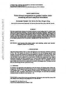
386 the time taken by the same problem on n processors. Figure 1 shows the variation of S with n. The scaling performance improves as one uses a more refined mesh. Mesh M5 is the most refined of all meshes. The flow solution on this mesh requires solving 369.9 million equations. As seen from Fig. 1, close to linear speedup is achieved on this mesh.

Sanjay Mittal et al. model. These are referred as model-free computations. The variation of CD with Re is presented in Fig. 2. Also shown are the well established experimental and computational results. The present results are in reasonable agreement with data from earlier studies. Fig. 2 shows that both 2D and 3D model free simulations predict the drag crisis phenomenon at a slightly lower Re compared to experimental results. This figure also highlights that drag crisis phenomenon is predominantly 2D, as the critical regime lies in the same Re regime in both two and three dimensions. However, for subcritical and supercritical regime three dimensional simulations, with NZ =51, provide a more accurate prediction of the values of CD . Figure 3 shows time and span averaged

Fig. 1: Speedup of parallel finite element code on HPC 2013 mac h in e

Drag Crisis in Flow Past a Circular Cylinder Drag crisis is sudden drop in the drag experienced by a body as the Re is increased beyond a certain critical value. For a smooth circular cylinder, the critical Re at which drag crisis occurs is 2x105, approximately. This phenomenon is associated with transition of boundary layer, from laminar to turbulent state. The turbulent boundary layer results in delay of flow separation over the surface of cylinder. This leads to increase in the base pressure and reduction in drag coefficient ( CD ). Roshko, 1961 categorized the flow past a smooth cylinder into four regimes: (i) subcritical:

CD is constant with Re and its approximate value is 1.2, (ii) critical: the drag crisis occurs in this regime, (iii) supercritical: CD reduces to nearly 0.3 and, (iv) transcritical: CD increases gradually with Re to 0.7, approximately. The present work looks into predicting and understanding the mechanism of drag crisis in flow past a circular cylinder via 2D and 3D simulations. The 3D grid was prepared by stacking Nz number of 2D grid sections in spanwise direction. Bulk of the simulations were carried out without any turbulence

streamlines ( ) and instantaneous spanwise vorticity (Z) at Re=5x104 and 3.5x105. These lie in subcritical and supercrtitical regimes respectively. Fig. 3 explains the mechanism of transition of boundary layer from laminar to turbulent state. At Re=5x104 the boundary layer undergoes laminar separation. The separated shear layer becomes unstable at a downstream location. At higher Re, for example at Re=3.5x105 the separated shear layer reattaches to the surface and separates at a larger angle. The reattachment of the shear layer as a turbulent boundary layer is due to the enhanced mixing provided by the shear layer vortices which are created by the destabilization of the separated shear layer very near to the cylinder (Singh and Mittal, 2005). This mechanism also leads to the formation of Laminar Separation Bubble (LSB) on the surface of cylinder. LSB can be seen in the time- and span-averaged streamlines (  ) of the Re=3.5x105 flow in Fig. 3(B). LSB is present on both the top and bottom surface of the cylinder, indicating that flow separation is symmetric. The delay in flow separation leads to narrower wake which causes the

CD to reduce. This can be observed from figure 3 where Re=5x104 flow has a wider wake compared to 3.5x105 flow. Clearly the appearance of LSB is vital to the transition of boundary layer from a laminar to turbulent state. More importantly, it was also found that process of transition and appearance of LSB is an intermittent process in the critical regime where drag crisis occurs. This is quantified using

Finite Element Computations of Complex Flows

387

Fig. 2: Flow past a cylinder: Variation of the mean drag coefficient with Reynolds number

(A)

(B)

Fig. 4: Flow past a cylinder: variation of the intermittency factor and mean coefficient of drag with Re Fig. 3: Flow past a cylinder: instantaneous pictures of spanwise vorticity (left) and time and span averaged streamlines (right) at (A) Re=5x10 4 and (B) Re=3.5x10 5

Intermittency factor (If). This is a well-established concept in turbulence where, intermittency represents the fraction of time a flow is in turbulent state. In the present work If represents the fraction of time an LSB is present in the flow. The value of If lies between 0 and 1, where 0 indicates LSB never appears in the flow while a value of 1 corresponds to the LSB being present at all times in the flow. The Intermittency factor is estimated from the root mean square (rms) of fluctuations of the coefficient of pressure (Cp) on the surface of cylinder. Fig. 4 shows the distribution

of 1-If and CD with Re. It can be observed from the figure that there is a very good correlation between 1-If and the mean coefficient of drag. In the subcritical regime, where the boundary layer undergoes laminar separation without reattachment, 1-If is one and the

CD is high. The LSB is never formed in this flow. In the critical regime when the drag reduces with increase in Re, 1-If also reduces. In the lower critical regime, the LSB begins to appear in the flow but exhibits an intermittent nature. This is reflected in the relatively large value of 1-If. On the other hand, towards the end of the drag crisis, 1-If approaches zero. This

388

Sanjay Mittal et al.

indicates that LSB is present in the flow at all times. This analysis clearly shows that the drag crisis and transition of boundary layer from laminar to turbulent state is a relatively gradual process spanning across the critical regime. The LSB does not appear suddenly at a certain Re; rather it appears intermittently with increased presence with increase in Re. Vortex Induced Vibrations (VIV) Unsteady aerodynamic forces resulting from vortex shedding in flow past bluff bodies may lead to its vibrations. If unattended, such vibrations may cause fatigue damage and in many cases lead to catastrophic failure of structures. Therefore, vortex-induced vibration (VIV) is considered as a problem of practical importance in several branches of engineering, e.g. oscillation of oil risers bringing oil from the sea bed. Recently, there has been surge in VIV studies because of its application in harvesting energy from the flow along the sea bed. The response of the structure undergoing free vibrations depends on many parameters. This research mainly focuses on exploring the effect of Re, shape and mass of the body, structural damping and natural frequency on VIV. An important phenomenon associated with VIV is lock-in/ synchronization/wake-capture. During lock-in, the structure exhibits large amplitude of oscillation. In this regime, the frequency of vortex shedding is different from the situation when the structure is stationary. We investigate VIV for the flow past bodies with different geometries over a wide range of Re. 2D and 3D computations are carried out depending on the flow regime. It is observed that the peak amplitude of oscillation increases with increase in Re (Navrose and Mittal, 2011). For low values of Re, the response of a circular cylinder is associated with two branches: initial and lower (Fig. 5). At large Re, a third branch called the upper branch appears (Fig. 6). The different branches of cylinder response are associated with different modes of vortex shedding. Each mode is associated with different level of fluctuations in the lift forces. The transition between different branches may be associated with hysteresis or intermittent switching. In general, the upper branch is associated with the largest fluctuation in lift force as well as the peak amplitude of cylinder oscillation. To investigate the effect of proximity of another body on free vibrations of a cylinder, computations are carried out with multiple cylinders in different configurations. The

Fig. 5: Flow past a freely vibrating cylinder in low Re regime: the two branches of cylinder response and the mode of vortex shedding at different Re (Navrose and Mittal, 2011)

Fig. 6: Flow past a freely vibrating cylinder at Re=1000: the three branches of cylinder response and the different modes of vortex shedding on the different branches (Navrose and Mittal, 2011)

size of the cylinders and the spacing between them in found to have significant impact on the response of the cylinder and the wake. The effect of finite eccentricity on VIV is also explored. It is observed that an elliptic cylinder with minor axis aligned parallel to the incoming flow experiences larger amplitude of oscillation compared to the situation where the major axis is aligned parallel to the flow. The aspect ratio is also found to affect the width of the lock-in regime. The effect of imparting rotation to the body is also explored. Such VIV scenarios are quite important for off shore drilling processes. With increase in the rotational speed, the peak amplitude of circular cylinder increases, reaching a value that is several times the diameter of the cylinder. The range of large amplitude oscillation increases with increase in the

Finite Element Computations of Complex Flows rate of rotation. Compared to its circular counterpart, VIV of square cylinder is found to be associated with higher amplitude of oscillation and richer vortex shedding patterns. Depending on the orientation of the square cylinder with respect to the incoming flow galloping oscillation can also occur alongside VIV. Fluid Structure Interaction of Cylinder With Splitter Plate Problems involving effect of fluid structure interaction (FSI) of flexible splitter plates on flow past circular and square cylinders are numerically studied. An opensource program, based on standard Galerkin descretization, Calculix, is employed for solving the structural dynamics equations. A block iteration based partitioned approach is utilized to couple the fluid and structure sub-problems. Furquan and Mittal, 2014 studied the flow past two rigid square cylinders with attached flexible splitter plates, placed side-by-side in a uniform flow. The Re of the flow is fixed at 100, while the flexibility of the plates, Ae, is varied. Initially, the plates exhibit small amplitude vibrations which are almost 180° out-ofphase with each other. The flow is symmetric about the centerline at this stage. However, this changes with time. Beyond a certain time, the plates begin to oscillate in phase. The fully developed oscillations are associated with large amplitude when the frequency of plate oscillations is close to the natural frequency of the plates. Fig. 7 shows an instantaneous vorticity field for both in-phase and out-of-phase oscillations for the case with Ae=8.05x105.

(A)

389 The effect of flexibility of the splitter plate on the vibration of an elastically mounted circular cylinder is studied at Re=150. When the splitter plate is relatively rigid, it is able to suppress the VIV of the cylinder. However, at large reduced speeds the galloping oscillations set in. The amplitude of oscillations is found to increase with increase in the reduced speed. Highly flexible plates, on the other hand, do not show galloping response but are less effective in controlling VIV of the cylinder. The study suggests that there exists an optimal value of flexibility to effectively control both VIV and galloping oscillations. Fig. 8 shows instantaneous vorticity field for the case of density ratio = 10, reduced velocity Us*=6 and Ae=44571.

Fig. 8: Instantaneous vorticity field for flow past an elastically mounted cylinder with an attached flexible splitter plate. The figure shows instantaneous vorticity field for Re=150, density ratio = 10, U s*= 6 and Ae=44571

Aerodynamic Shape Optimization in Fluid Flows using Adjoint Approach Shape optimization in fluid mechanics is on its way to becoming an integral part of the design process. Srinath and Mittal, 2010 formulated and implemented a (B)

Fig. 7: Instantaneous vorticity field for flow past two side-by-side square cylinders with attached splitter plates for Re=100 and Ae=8.05x10 5 showing (A) out-of-phase oscillations during the initial stage of the solution, (B) fully developed in-phase oscillations (Furquan and Mittal, 2014)

390


continuous adjoint-based method for shape optimization in steady low Re flows. This method was utilized to design optimal airfoils at low Re. Adjoint methods are most effective in optimization as the cost of computing the gradients or sensitivities are independent of the number of design variables (Kumar et al., 2013). The shape of the body is parametrized via a Non-Uniform Rational B-Splines (NURBS) curve and is updated by using the gradients obtained from solving the flow and adjoint equations. The adjoint equations are also solved using SUPG and PSPG methods. The L-BFGS algorithm is employed to minimize the objective function and provide a new search direction depending on the gradients. Shape optimization was extended to unsteady flows by Srinath and Mittal, 2010 for airfoil at Re = 10,000. Interesting shapes are obtained with NACA 0012 as initial guess, especially when the objective is to produce high performance airfoils. Fig. 9(A) shows the airfoil obtained for an inverse coefficient of lift = 0.75 and (B) coefficient of pressure distribution for Re = 1000 flow at  = 4o. There is an increase in lift of 275 % compared to the initial guess. The effect of corrugations on the aerodynamic performance of a Mueller C4 airfoil, placed at a 5° angle of attack, at Re=10,000 was investigated by Sambhav et al., 2015. The computations were carried out for different location and number (n) of corrugations while keeping the height of the corrugation (h=1.5%c) fixed. PTOC (Preserve thickness, optimize camber) optimization strategy was used to obtain the highest lift coefficient and aerodynamic efficiency of 0.997 and 16.9, respectively. This is 42 % and 7% higher than Mueller C4 airfoil. The optimal shape is shown in Fig. 10(B). Elliptic and rectangular planforms were

Fig. 10: Pressure distribution for flow past (A) Mueller C4 airfoil and (B) Optimal airfoil obtained through PTOC strategy (Sambhav et al., 2015)

optimized for Re=1000 based on root chord and  = 4o to the oncoming flow by Kumar et al., 2013. A 3D wing is parametrized by a control net, obtained by stacking control polygons at different of spanwise locations. Biparametric tensorial NURBS surface is interpolated on the control net to generate the wing surface. Fig. 11 shows the control net and the resulting NURBS surface for a wing with elliptic planform. Fig. 12 shows the comparison of planform shapes and Fig. 13 shows iso-surface of the streamwise component of vorticity ( x = –0.3) for all the planforms. The length of the wing-tip vortex is longer for the rectangular and elliptic planform whereas it is shorter for the optimal shape with an additional weak vortex at the winglet type structure near the wing-tip. The optimal shape has 15 % increase in aerodynamic efficiency compared to the other planforms. Supersonic Flow in Air Intakes The purpose of an air-intake is to capture free-stream air and bring it to an optimal condition desired by engine. In the case of a supersonic aircraft, this is achieved by a design that slows the flow via a train of oblique shock waves, followed by a weak normal shock. In this study, Y-intake and mixed compression air intakes are considered. Flow in Y-intake configuration was studied by Kotteda and Mittal, 2015.

Fig. 9: Inverse design of airfoil for coefficient of lift = 0:75 at Re = 1000,  = 4 o : (a) initial and optimal shapes and (b) timeaveraged coefficient of pressure distribution on surface (Srinath and Mittal, 2010)


391

Fig. 11: Representation of an elliptic wing at  = 4 o with a NURBS surface (Bhatt et al., 2015)

Fig. 12: Comparison of planforms shapes for Re = 1000 flow at  = 4o (Bhatt et al., 2015)

The Y-intake configuration is used in many modern supersonic fighter aircrafts with single engine which have high manoeuvrability. The computations are carried out at M=1.5 with different back pressure ratios (pb/pi) and sideslip angles (). The performance of the intake is studied for 2.1 < pb/pi d < 3.5 and 0o <  < 5o. The onset of buzz instability in the intake is observed at pb/pi = 3.276 for =3o. It is shown in Fig. 14. The first three frames show a buzz cycle. In the first and last flow frames, the bow shocks are at their most downstream locations while they are at their

Fig. 13: Comparison of iso-surfaces of streamwise vorticity for (a) rectangular, (b) Elliptical, and (c) optimal planform for Re=1000 flow at  = 4o (Bhatt et al., 2015)

392


Fig. 14: M=1.5, Re=1x10 5,  = 3 o, pb/pi = 3.276 flow in the Y-intake at various time instants during onset of instability. Time histories of the mass flow rate in the top and bottom limb (left) and pressure at the middle of the top and bottom limb (right) at the merger section are shown in the last row. The time instants at which the flow is shown are marked on these plots (Kotteda and Mittal, 2015)

most upstream location in the second frame. The net flow in the bottom limb is always positive. However, the top limb experiences a reverse flow during part of the buzz cycle as also seen in the time history of the mass flow rate. Streamlines as well as vorticity fields are shown in the right column of Fig. 14. The upstream movement of the bow shock can be seen in second frame. It is accompanied with an upstream movement of the vortex, located in the duct beyond the merger section, and the reverse flow in the top limb. The negative mass flow rate in the top limb corresponding to the second frame can be seen in the time history. The bow shocks upstream of the top and bottom limbs move back and forth leading to very

large amplitude oscillations in the mass flow rate delivered to the engine face. The buzz cycle is fairly periodic and repeats itself. Interestingly, the net mass flow rate through the intake is still positive and the engine continues to receive air flow, but at a reduced level. Cellular Oblique Vortex Shedding It is well known that due to the end wall effects, the vortex shedding past a cylinder is associated with vortices oblique to the axis of the cylinder. Another feature due to the presence of the walls is the formation of a cellular structure of the vortices along the span. The present work focuses on the analysis


A

B

C

Fig. 15: Flow past a three dimensional cylinder with end walls: instantaneous spanwise vorticity for (A) onecell, (B) two-cell and (C) three cell shedding patterns

of flow past a 3D circular cylinder at low Re in the laminar flow regime. Three key parameters have been identified that characterize the flow - Aspect Ratio (AR) of the cylinder, Re and boundary condition at the cylinder ends. The aim of the study is to characterize the flow in the parameter space of AR and Re, and attempt to understand the reasons that lead to cellular shedding. In this study, numerical simulations have been carried out to simulate flow past a wall bounded finite cylinder to study the effect of each parameter. Computations have been carried out for 10