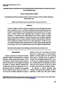
Response surface methodology using Gaussian processes: towards optimizing the trans-stilbene epoxidation over Co2+-NaX catalysts Qinghu Tang, Ying Bin Lau, Shuangquan Hu, Wenjin Yan, Yanhui Yang, Tao Chen* School of Chemical and Biomedical Engineering, Nanyang Technological University, Singapore 637459, Singapore Abstract: Response surface methodology (RSM) relies on the design of experiments and empirical modelling techniques to find the optimum of a process when the underlying fundamental mechanism of the process is largely unknown. This paper proposes an iterative RSM framework, where Gaussian process (GP) regression models are applied for the approximation of the response surface. GP regression is flexible and capable of modelling complex functions, as opposed to the restrictive form of the polynomial models that are used in traditional RSM. As a result, GP models generally attain high accuracy of approximating the response surface, and thus provide great chance of identifying the optimum. In addition, GP is capable of providing both prediction mean and variance, the latter being a measure of the modelling uncertainty. Therefore, this uncertainty can be accounted for within the optimization problem, and thus the process optimal conditions are robust against the modelling uncertainty. The developed method is successfully applied to the optimization of trans-stilbene conversion in the epoxidation of trans-stilbene over Co2+-NaX (cobalt ion-exchanged faujasite zeolites) catalysts using molecular oxygen. Keywords: Design of experiments; Gaussian processes; Heterogeneous catalysis; Latin hypercube sampling; Optimization; Response surface methodology. 1. Introduction Response surface methodology (RSM) is a family of statistical techniques for the design, empirical modelling and optimization of processes, where the responses of interest are influenced by several process variables (termed factors) [1,2]. RSM comprises the following three major components: (i) experimental design to determine the process factors’ values based on which the experiments are conducted and data are collected; (ii) empirical modelling to approximate the relationship (i.e. the response surface) between responses and factors; and (iii) optimization to find the best response value based on the empirical model. In addition, the above three-stage procedure is typically operated in an iterative manner, where the information attained from previous iterations is utilized to guide the search for better response variables. This iterative exploration of experimental space has been adopted and applied in various model-based process optimization methods, such as those using genetic algorithms [3-5], and “active sampling” [6] that was originally developed in the machine learning society [7]. RSM is particularly applicable to problems where the understanding of the process mechanism is limited and/or is difficult to be represented by a first-principles mathematical model. Depending on specific objectives in practice, these RSM techniques differ in the experimental design procedure, the choice of empirical models, and the mathematical formulation of the optimization problem. An appropriate design of experiments (DoE) is the pre-requisite for a successful experimental study. The classical fractional factorial and central composite designs were proposed to investigate the interactions of process factors based on polynomial models [2]. These classical designs typically assign two or three predetermined levels for each process factor, and experiments are conducted at the combination of the levels of different factors. Using a small number of levels is especially appealing if the factors’ values are difficult to change in practice. However, this strategy may not have an optimal coverage of the design space due to limited levels of the factors being studied, and thus it may result in a less reliable empirical model [8]. The recognition of this disadvantage of classical DoE methods has motivated the concept of “space-filling” designs that allocate design points to be uniformly distributed within the range of each factor [8-10]. Among this class of designs, the Latin hypercube sampling (LHS) [9] is probably the most widely adopted method as a result of its simple implementation and good performance. For this reason, LHS is a preferred method in practice, and it is adopted for experimental design in this study. There has been considerable effort to improve the LHS to obtain *
Corresponding authors. Tel.: +65 6513 8267; Fax: +65 6794 7553 (T. Chen). Email addresses:
[email protected] (T. Chen).
1
more uniform design points [8,10] although improving the uniformity is at the expense of significantly higher computation. After experimental data are collected according to the design points, the next step of RSM is to develop an empirical model for the response surface. The traditional method is to fit a polynomial function (typically linear, quadratic or cubic polynomial) to the data, followed by identifying the factor values that optimize the objective function. However, the prediction accuracy of the empirical model is usually unsatisfactory when using polynomial functions, and consequently the identified optimum is unreliable. To address this issue, artificial neural network (ANN) was proposed to provide a more accurate approximation of the response surface, and it was demonstrated to give improved optimization results in various applications [11-16]. More recently, ANN has been combined with other methods, such as genetic algorithm, principal component analysis and clustering analysis, for modelling, analysis and optimization of various catalysis systems [3-5,1719]. An alternative approach is support vector machine (SVM) that belongs to the family of kernel modelling methods [20]. SVM employs a structural risk minimization scheme to improve the prediction accuracy, and it has been successfully applied to predictive modelling of catalysis processes [21,22] and other chemical systems [23]. The primary purpose of this study is to apply Gaussian process (GP) regression as the empirical model for RSM. GP models have recently received considerable attention in process systems engineering and chemometrics [24-26]. GP can be viewed as an alternative approach to ANN because a large class of ANNbased Bayesian regression models converge to GP in the limit of an infinite network [27]. GP models can also be derived from the perspective of Bayesian regression [28], by directly placing Gaussian prior distribution over the space of regression functions. The fact that GP models attain both good practical performance and desirable analytical properties motivates the current work, where the polynomial function or ANN is replaced by GP for process optimization. In addition to prediction accuracy, GP models are also known for the capability of providing reliable prediction variance, which measures the uncertainty of the studied model, i.e. the degree to which the model is not sure about its prediction [27-29]. As a consequence, the model-based optimization problem can be formulated to account for the uncertainty, and the identified optimal process factors are expected to be more robust against modelling uncertainty. The major contribution of this work is two-fold. First, we propose the application of GP, in place of traditional polynomial regression and ANN, for process modelling so that the model uncertainty can be handled. Second, we extend previous non-iterative GPbased RSM [30,31] to an iterative approach, whereby the GP model is used to help search for the best process performance incrementally. In this sense, the proposed approach falls in the category of “active sampling” methods to iteratively allocate experiments with the aid of a model to explore the design space, so that the optimal process conditions are identified [6,7]. In a broader literature, GP regression has been applied to mechanical system optimization [30], and notably used as “metamodel” for the optimization of complex functions and computer models [31-33]. The predictive uncertainty obtained by GP was utilized in various ways. Apley et al. [31] considered a “worst-case scenario” and proposed to maximize the statistical lower bound. More elegant criteria were discussed by Jones [32] to optimize the “probability of improvement” or “expected improvement”. As the name suggests, metamodel is to approximate another complex computer model using a GP, whilst in the current study we are concerned with approximating and optimizing a real chemical process. Although the methodology for optimizing a computer model and a real process is largely similar, there is a salient distinction between them. Specifically, computer model itself is an approximation of the real process. As a result, in order to apply the optimal conditions obtained from a complex model to a real process, additional uncertainty resulting from the mismatch between the computer model and reality has to be accounted for; see [29] for a comprehensive discussion on this matter. In this paper, we restrict our scope to the development of RSM for the optimization of real chemical processes. Of particular interest in this study is the catalytic oxidation process that converts trans-stilbene into stilbene oxide using molecular oxygen as the oxidant. Stilbene oxide is a commercially important intermediate used in the synthesis of various fine chemicals and pharmaceuticals. Conventionally, stilbene oxide is produced using organic peracid as an oxidant or by a chlorohydrin process, and a large amount of chemical waste is formed [34]. As a consequence, it is desired to exploit molecular oxygen or air as oxidant for stilbene epoxidation from the environmental, safety and economic considerations. Recently, cobalt ion-exchanged faujasite zeolite (Co2+-NaX) has been reported as an efficient heterogeneous catalyst for the epoxidation of trans-stilbene using O2 in the absence of co-reductant [35,36]. These reports focused on the synthesis of catalyst and catalytic performances; studies on the process of the epoxidation are limited. Therefore, it is of great importance to 2
optimize the existing catalytic oxidation process, through investigating the effect of the process factors on the overall performance (response). Traditionally, heterogeneous catalysis research heavily relies on tedious experimental studies, screening a large number of process factors that may affect the reaction performance. Despite the wide acceptance of RSM in various scientific disciplines, the usual “one-factor-at-a-time” approach is still common in catalysis research. That is, one factor is varied each time, with others being fixed, to investigate individual factor’s influence on process performance. This “one-factor-at-a-time” method ignores the interactions between different factors, and has long been criticized of having little chance (if any) of finding the optimal conditions [3-6,11-19,37]. As a consequence, the current work serves a dual purpose: to propose a novel GP-based RSM framework, and to demonstrate/validate its application in an important catalytic reaction process. A remarkable advance in recent catalysis research is the emergence of high-throughput experimentation (HTE) that is capable of conducting hundreds of experiments within a relatively short period of time [38,39]. Given the large amount of data, a proper DoE and data-based modelling methodology is crucial to guide the search for optimal catalysts. Some afore reviewed computational procedures, such as ANN, SVM and their combination with genetic algorithm, have been adopted and adapted to aid catalyst design [4,17,18,40-42]. In this paper, we will focus on the situation where HTE is not available, as is the case in many traditional laboratories or industrial processes, and thus a relatively small amount of data can be collected. Previous studies have suggested that when data are limited, GP regression models are especially superior to other techniques in terms of prediction accuracy [43]. Another related field where data-based modelling is widely applied is quantitative structure activity and property analysis (QSAR and QSPR). Originally emerged from drug discovery, QSAR/QSPR aims to relate the structural descriptors of certain molecules to their effectiveness in curing certain diseases. In the context of heterogeneous catalysis, the descriptors typically include catalyst composition, tabulated physico-chemical properties, and catalyst synthesis and reaction conditions [44]. Given such large number of descriptors (up to several thousand), HTE is typically needed to obtain sufficient data for a reliable analysis, and thus this topic is outwith the scope of the current study. The rest of this paper is organized as follows. Section 2 gives a brief description of the catalytic trans-stilbene oxidation process. Section 3 presents the proposed RSM framework, including four major components: the LHS method for experimental design, the GP model for approximating the response surface, model-based “region-searching” (to be presented subsequently) and model-based optimization. To facilitate the adoption of the proposed methodology, the software tools to implement the RSM framework are either made freely available (if written by the authors) or identified through relevant links. Results and discussions are given in Section 4, followed by concluding remarks in Section 5. 2. Experimental In this study, a lab-scale catalytic reaction is utilized as a test-bed to validate the proposed RSM technique. Specifically, we are interested in maximizing the trans-stilbene conversion rate in the epoxidation of transstilbene over Co2+-NaX catalyst using molecular oxygen as the oxidant. Five process factors are considered: reaction temperature, partial pressure of oxygen, initial trans-stilbene concentration, stirring rate and reaction time. The range of these factors to be explored is listed in Table 1. (Table 1 about here) Sodium form Zeolite X (NaX) was purchased from Sigma-Aldrich. Unit cell composition of NaX was Na88Al88Si104O384 with unit cell dimension of 24.94 Å. The BET surface area of the zeolite was 608 m2·g-1. Cobalt-exchanged zeolite (Co2+-NaX) was prepared by ion-exchange of the NaX with 0.1 M Co(NO3)2 aqueous solution with 1:80 ratio of NaX zeolite to Co(NO3)2 followed by heating at 80 °C for 4 h. The resulting powder was filtered and washed with deionized water until it is free from unexchanged cobalt ions. The washed Co2+-NaX sample was dried at 100 °C for 4 h. The liquid phase catalytic trans-stilbene epoxidation reactions were carried out using a batch-type reactor operated under atmospheric pressure. In a typical reaction, a measured amount of trans-stilbene (> 96%, Aldrich), 200 mg of Co2+-X catalyst, and 15 ml of N,N-dimethylformamide (DMF, > 99.8%, J.T.Baker) 3
were introduced into a 50 ml round-bottomed flask followed by bubbling O2 or O2 diluted with N2 into the liquid at a flow rate of 50ml· min-1 . The reaction was initiated by immersing the round bottom flask into an oil bath under desired reaction temperature. The solid catalyst was filtered off after reaction, and the liquid organic products were analyzed by an Agilent gas chromatograph (GC) 6890 equipped with a HP-5 capillary column (30 m long and 0.32 mm in diameter, packed with silica-based supel cosil). Calibration of GC was done using solutions with known amounts of benzaldehyde, benzoic acid, stilbene, and stilbene oxide in DMF. The conversion was calculated on the basis of moles of stilbene as follows:
Conversion (%) =
(initial moles) - (final moles) × 100% (initial moles)
(1)
During experimentation, the process factors were accurately controlled to minimize the process variability. In addition, the Co2+-NaX catalyst used in the experiments was from the same batch to avoid variation due to catalyst preparation procedure. As a result, our preliminary study showed that by conducting multiple experiments at the same value of the process factors, the standard deviation of the conversion rates is typically within 1%. Therefore, the process variability does not significantly affect the response and will not be considered further. In a more practical scenario where the factors and/or catalysts cannot be closely controlled, robust design and optimization methodology would be needed, which is an interesting future research direction. 3. Response surface methodology using Gaussian processes The proposed RSM framework is operated in an iterative manner and is summarized step by step as follows. Step 1: Use LHS to obtain design points that are uniformly distributed over the entire factor space. Step 2: Conduct experiments at the design points, and collect the response data. Step 3: Develop a GP regression model, using all the experimental data collected up to the current iteration, to approximate the response surface. Step 4: If this is NOT the final iteration Then: (a) Find the region of factors that is predicted (using the GP model) to give a better response variable. (b) Use LHS to allocate design points that are uniformly distributed over this region, and go to Step 2 for the next iteration. Else: (c) Solve the mathematical optimization problem based on the GP model to obtain the optimal values of the process factors. (d) Conduct final experiment(s) to validate the optimal conditions. In the initial iteration, little knowledge is available regarding the factors’ values for desirable response variables, and thus LHS will be used to uniformly fill the entire factor space with designed points (Step 1). At Step 2, actual experiments will be conducted carefully at the design points to obtain the corresponding response variables, followed by Step 3 to develop a GP model to approximate the relationship between the response and process factors. In Step 4, if this is not the final iteration, a model-based approach is used to identify the region of factors that is more likely to produce better responses (Step 4(a)), followed by using LHS to generate design points within this region for experiments in next iteration (Step 4(b)). Step 4(a) is referred to as “region-searching” in this paper. After several iterations of this procedure, the factor space has been well explored and no more iterations are needed. In this case, Step 4 is to use a model-based optimization approach to obtain the optimal values of the process factors (Step 4(c)), followed by the final experiment to validate the optimal conditions (Step 4(d)). Conceptually, this iterative procedure is similar to the traditional catalyst screening practice. However, the conventional methods search for region-of-interest purely based on experimental data and intuition [44]. In contrast, the proposed strategy takes advantage of a GP model to predict a better region of factor’s values. Therefore, RSM is a rational, as opposed to trial-and-error, approach to process optimization. We discuss each individual step within an iteration in more detail below. 3.1. Experimental design through Latin hypercube sampling 4
The key objective of DoE is to select the values of process factors in such a way that the obtained experimental data are representative of the design space being explored and informative to predict the process responses. This section presents a specific DoE method, Latin hypercube sampling (LHS) [9], and its incremental algorithm. LHS is a special “space-filling” DoE method that selects the factors’ values to be uniformly distributed. As a result, the data will be more representative of the entire design space than the classical factorial and central composite designs. It was shown that LHS is more efficient than randomly generating the uniform samples from the design space. For the same number of design points, the modelling and estimation accuracy of LHS is substantially better than those of random sampling [9]. Specifically, let Rk (k = 1,K , K ) be the range of values of factor k and N be the number of design points to be generated. The first step of LHS is to divide the range of each factor k, Rk, into N equally spaced intervals, followed by uniformly sampling from each interval to result in N values for this factor: xkj , j = 1,K , N . Subsequently, these N values are randomly permuted to have a better coverage of the design space. This procedure is repeated for all the K process factors to attain K × N values: xkj , k = 1, K K , j = 1,K, N , which form the N design points, each being K dimensional. More details of LHS can be found in [9]. The LHS algorithm has seen applications in various disciplines, partly due to its relatively simple implementation and its wide availability in statistical software packages (e.g. Statistical Toolbox for Matlab). The capability to incrementally increase the design points is clearly a desired property of LHS, and other DoE methods, since RSM is often conducted iteratively. A straightforward approach is to apply the LHS algorithm multiple times to add more design points without any consideration of previous data. However, although LHS guarantees that each set of points are located in the equally spaced N intervals at each dimension, the entire data set does not necessarily cover the design space uniformly. We illustrate this phenomenon in Fig. 1 in which a single process factor is considered. Initially, two design points are generated and located in two equally spaced intervals (Fig. 1(a)), followed by adding two more design points. If these two new data are generated by repeating LHS algorithm, it only guarantees that the new points are separately located in the original two intervals; however, they can be close to the original data and thus undesirable (Fig. 1(b)(c)). To address this issue, we adopt a simple but efficient incremental approach for LHS [45]. Suppose N1 design points were previously generated by LHS and N2 additional points are required, the incremental algorithm divides the range of each factor into (N1 +N2) equal intervals. Clearly, at least N2 of the intervals do not contain any previous data. It is possible that there are more than N2 empty intervals due to more than one data point falling into the same interval. Therefore, we randomly select N2 empty intervals and generate a random sample from each of them. The above procedure is repeated for each factor to attain N2 new design points. Note that the incremental algorithm does not guarantee that all (N1+N2) design points are allocated into (N1+N2) equally spaced intervals because some intervals may not be occupied if there are more than N2 empty intervals. Nevertheless, this algorithm is a fast and efficient way to obtain significantly better coverage of the design space than repeated LHS. A Matlab implementation of the incremental LHS algorithm is available from: http://www.ntu.edu.sg/home/chentao/. (Fig. 1 about here) 3.2. Gaussian process regression modelling The idea of Gaussian process (GP) can be dated back to the classical statistical method by O’Hagan [46]. However, the application of GP as a regression (and classification) technique was not common until late 1990’s, when the rapid development of computational power facilitated the implementation of GP for large data sets. Recently, GP models have seen successful applications in various fields, including chemometric calibration of spectrometers [24], chemical process modelling [25,47], prediction of biological binding affinities [26], and mechanical system modelling and optimization [30]. In this subsection, a brief overview of GP regression technique is given, including the formulation and implementation of the model. From the perspective of a regression problem, a functional relationship is identified between the K dimensional predictor variables (factors), x, and the response y. Consider a training data set of size N: {x i , yi ; i = 1, K , N } that was obtained by conducting experiments on the designed points. A GP regression model is defined such that the regression function y(x) has a Gaussian prior distribution with zero mean, or in discrete form: 5
y = ( y1 ,K, y N ) T ~ G (0, C)
(2)
where C is an N×N covariance matrix of which the ij-th element is defined by a covariance function: Cij = C ( x i , x j ) . An example of such a covariance function is: K K C (x i , x j ) = a0 + a1 ∑ xik x jk + v0 exp − ∑ wk ( xik − x jk )2 + σ 2δ ij k =1 k =1
where
(3)
xik is the k-th variable of x i , and δ ij = 1 if i=j, otherwise δ ij = 0 . We term
θ = ( a0 , a1, v0 , w1,K , wK , σ 2 )T “hyper-parameters” defining the covariance function. The hyper-parameters must be non-negative to ensure that the covariance matrix is non-negative definite. For the covariance function given in Eq. (3), the first two terms represent a constant bias (offset) and a linear correlation term, respectively. The exponential term is similar to the form of a radial basis function, and it takes into account the potentially strong correlation between the responses with similar predictors. The term σ 2 captures the random error effect. By combining both linear and non-linear terms in the covariance function, GP is capable of handling both linear and non-linear data structures [24]. Other forms of covariance functions are also discussed [28]. For a new data point with predictor vector x*, the predictive distribution of the output y* conditional on the training data is also Gaussian, of which the mean ( yˆ * ) and variance ( σ y2ˆ* ) are calculated as follows:
yˆ * = k T ( x* )C−1y
(4)
σ = C ( x , x ) − k ( x )C k ( x ) 2 yˆ *
*
*
T
*
−1
*
(5)
where k (x* ) = [C (x* , x1 ),K , C (x* , x N )]T . The hyper-parameters θ can be estimated by maximizing the following log-likelihood function:
1 1 N L = log p (y | θ, X) = − log | C | − y T C −1y − log(2π ) 2 2 2
(6)
This is a non-linear optimization problem which can be solved by using gradient based methods, e.g. the conjugate gradient method [28]. These methods require to calculate the derivative of log-likelihood with respect to each hyper-parameter θ , which is:
∂L 1 ∂C 1 T −1 ∂C −1 = − tr C −1 C y + y C ∂θ 2 ∂θ 2 ∂θ
(7)
where ∂C/∂θ can be obtained from the covariance function. A Matlab implementation of the GP models is publicly available from http://www.gaussianprocess.org/gpml/code/matlab/doc/, and it was used to produce the results in this study. It should also be noted that the calculation of the likelihood and the derivatives involves a matrix inversion step and takes time of the order O(N3), which can be extremely demanding for large data set. Fortunately in the context of RSM, the experiments are costly to run, and the available data are normally limited and should not pose a computational problem for GP modelling. In addition, for large data sets, sparse training strategies may be employed to significantly reduce the computational cost [48]. 3.3. Model-based region-searching
6
The GP model that relates the process response y to the factors x provides the basis to guide the search for more promising process factors, referred to as “region-searching” in this study. Once a better region of factors is identified, the LHS method will allocate new design points to this region for next-iteration experiments. In this stage, model robustness emerges as an issue because of the predictive errors (and thus uncertainty) that are inevitable when using a statistical regression model. The predictive uncertainty must be considered and accounted for in order to identify a trustworthy optimal region. Fortunately, GP models are capable of giving the uncertainty (through variance) of the prediction in addition to a mean predicted value, and the uncertainty should be incorporated into the region-searching method. In this paper the worst-case scenario is considered to deal with the prediction uncertainty. Suppose the objective is to maximize the response variable, we instead maximize the lower-bound of the response predicted by the GP model. Similar approach was adopted in [31] for the optimization of computer simulation of mechanical systems. Mathematically we seek to obtain the region of process factors defined by:
{x : yˆ (x ) − 1.645σ y ( x ) > c AND σ y ( x ) > b AND x ∈ S}
(8)
where yˆ (x ) and σ y (x ) are the predictive mean and standard deviation obtained from the GP model (Eqs. (4)(5)), respectively, and S denotes the range of the process factors as given in Table 1. Since the prediction from GP is Gaussian distributed, yˆ ( x ) − 1.645σ y ( x ) corresponds to the 95% lower-bound of the prediction, and c is a user-chosen value. Essentially, this is to search for the factors such that the 95% lower-bound of the response is greater than c. Furthermore, the constraint σ yˆ ( x ) > b is to avoid allocating design points to wellexplored region, where the GP model is quite certain about its prediction (i.e. with small σ y (x ) ) and thus further experiments in this region are not necessary. The proper value of b and c should be adjusted at each iteration based on the information from experimental data. The specific choice of b and c in this study will be discussed in the next section. Clearly there are an infinite number of design points that satisfy Eq. (8). Hence the region-searching essentially becomes a constrained DoE problem, where the factors’ values are selected to be uniformly distributed in the constrained space that is defined by Eq. (8). This constrained DoE problem can be solved as follows. Suppose from previous iterations, N design points were used and the experiments were conducted, and now N1 new design points are to be generated. Then we can generate N1 design points using incremental LHS algorithm (discussed in §3.1), and find the points such that Eq. (8) holds. Suppose n out of N1 points satisfy this constraint, and thus we can further generate N1-n design points using incremental LHS. This procedure is repeated until a total of N1 design points satisfy the above constraint, and these points are selected for the experiments in next iteration. The proposed procedure is an effective solution to the constrained DoE problem, since the incremental LHS algorithm ensures a uniformed distribution of the design points within the entire factors’ range ( x ∈ S ), and thus the points selected will also be uniformly distributed within the region given by Eq. (8). 3.4. Model-based optimization Once the factors’ space is well explored through several iterations of the RSM technique, the final step is to conduct the optimization of the response variable. Similar to region-searching step, the optimization problem is formulated to maximize the 95% lower bound of predicted response variable, subject to the constraint on the factors’ range ( x ∈ S ):
max ( yˆ (x ) − 1.645σ y (x )) x
s.t. x ∈ S
(9)
If process factors take continuous values within the range, classical algorithms (e.g. sequential quadratic programming and trust-region method) for solving non-linear constrained optimization problem can be used [49]. However, in practice Eq. (9) is typically a mixed-integer optimization problem, i.e. continuous process factors are coupled with categorical and discrete (or integer) factors. For example in the reactor available in our laboratory, the stirring rate is fixed to seven different values (200, 300, 400, 500, 700, 1000 and 1250 rpm, see Table 1) due to instrument constraint, and thus the stirring rate can only take a discrete set of values. When 7
a subset or all of the process factors are discrete, more advanced methods are needed, such as genetic algorithms [3-5] and branch-and-bound method [49]. Note that these advanced methods are also applicable for optimizing continuous factors. In this study, a branch-and-bound algorithm was developed under Matlab computational environment. A comprehensive optimization toolbox for Matlab (i.e. TOMLAB: http://tomopt.com/tomlab/) is commercially available and could also be used for solving this problem. 4. Results and discussions This section demonstrates the application of the proposed RSM framework for the optimization of stilbene conversion of a catalytic oxidation process. In the initial iteration, the knowledge about the process is relatively limited, and the LHS algorithm is used to obtain 20 design points within the whole range of five factors for experiments. The designs and corresponding stilbene conversion rates are given in Table 2. (Table 2 around here) Following the reaction experiments, the response surface is approximated by a GP model. Before the model is applied for subsequent region-searching or optimization purpose, its predictive capability should be assessed by the well-known cross-validation procedure [14,18,21,22]. In this study, we adopt the method of leave-oneout cross-validation (LOOCV) [50] to validate the GP regression model. LOOCV takes a single data point from the entire data set as the validation data, and then develop a GP model using the remaining data points. Hence the error for the validation data can be calculated. This procedure is repeated such that each data point is used once for validation, and the overall validation error (typically in terms of root mean squared error (RMSE) or coefficient of determination (R2)) is used as the criterion to assess model quality. In addition, to consider the effect of prediction uncertainty, we also use the average negative log predictive density (NLPD) [51] defined by
NLPD = −
1 N
N
∑ log p( yˆ (x ) = y | x ) i
i =1
i
i
(10)
to assess the prediction performance. When prediction is Gaussian distributed with mean yˆ ( x i ) and variance
σ 2yˆ (x i ) , p ( yˆ ( x i ) = yi | x i ) corresponds to the calculation of a normal density function with mean yˆ (x i ) − y i
and variance σ 2yˆ ( x i ) . NLPD reaches its minimum if all predictions are equal to the true value and the predictive variances are zero. It was shown [51] that given a prediction, the optimal variance is the squared error of the prediction mean. Therefore, NLPD penalizes both over-confident (small variance) and underconfident (large variance) predictions, and it is a reliable criterion to quantify the prediction quality under uncertainty. For the purpose of comparison, a conventional multiple quadratic polynomial regression model with stepwise variable selection is also developed [37]. Fig. 2 gives the prediction results of LOOCV for both GP and quadratic regression model. Clearly, the GP model (RMSE=5.42, R2=0.85, NLPD=6.07) has attained significantly higher prediction accuracy than the quadratic regression (RMSE=7.66, R2=0.70, NLPD=8.52). A final GP model is then developed from all the available data, and this model will be used for either regionsearching or optimization subsequently. (Fig. 2 around here) Table 2 and Fig. 2 also indicate that most experiments did not result in satisfactory conversion rate of stilbene. Indeed, only four experiments attained conversion rates higher than 15%. Therefore, it may be premature to claim that the optimal region has been well identified for process optimization. However, these experiments do provide important information as to which region of the factors’ space is more promising to improve the conversion rate. Following the region-searching algorithm presented in §3.3, we search for a new set of design points x such that the 95% lower-bound prediction from the GP model is sufficiently large (i.e. yˆ (x ) − 1.645σ yˆ (x ) > c ) and the prediction uncertainty is also large ( σ yˆ (x ) > b ). The choice of b and c is 8
subject to the experimenter’s discretion. Based on the experimental results obtained in iteration 1, it may be reasonable to set c=15%, in the hope to explore the factors’ region with conversion higher than 15%. In addition, we set b to be the average standard deviation of predictions in the LOOCV procedure, so that to generate design points that are not well predicted by the current model. Based on these choices, the incremental LHS algorithm generates a new set of 20 design points as shown in Table 3, which also lists the conversion rates obtained through reaction experiments. (Table 3 around here) A comparison between Tables 2 and 3 confirms that the RSM framework has successfully identified more promising region of the process factors. On average, the conversion rate of the 20 experiments in Table 3 is 34.76%, which is a dramatic improvement over the average conversion of 11.04% in Table 2. The maximal conversion achieved in Table 3 is 61.05%, as opposed to 55.00% in Table 2. In addition, recall that the objective of the region-searching in iteration 1 is to find the process factors with conversion higher than 15%. This objective has been fulfilled for most experiments in Table 3, except the 15th and 17th runs (conversion rate of 7.52% and 12.29% respectively). Therefore, it appears that the GP model is reasonably reliable for predicting the process response variable. In principle, the RSM can be iterated multiple times as required, and the number of iterations should be decided by the experienced experimenters after careful examination of the results. The primary purpose of the present study is to demonstrate and validate the proposed RSM framework, and thus the number of iterations is restricted to two. Indeed, the specialists in catalytic reactions also feel that the identified factors in Table 3 may be close to the optimal condition achievable given the current experimental environment. To enable the optimization in the final iteration, a new GP regression model is required to approximate the response surface, using all the 40 data points available in Table 2 and 3. Again, the LOOCV approach is employed to assess the prediction capability of GP and conventional quadratic regression models, and the prediction results are shown in Fig. 3. With more data available in iteration 2, the prediction accuracy of both GP and quadratic models has been improved in comparison with iteration 1. Adding more data typically has significant effect on reducing the prediction error in RSM, since initially the data are very limited. However, due to the time and cost associated with experiments, it may be unrealistic to request a large amount of experimental data to be collected in the process design and development stage. Therefore, advanced modelling approaches should be utilized if they can provide more accurate predictions than conventional methods on the same amount of data. Fig. 3 indicates that, again, the GP model (RMSE=3.77, R2=0.96, NLPD=3.06) is superior to the quadratic regression (RMSE=5.31, R2=0.92, NLPD=3.60) in terms of lower RMSE, higher R2 value and lower NLPD values. Furthermore, a paired t-test on absolute prediction errors gives a p-value of 0.006, indicating that the improved accuracy of GP is statistically significant. (Fig. 3 around here) Based on the finally developed GP model from all the 40 experimental data, the optimization problem defined in Eq. (9) is solved using branch-and-bound algorithm. The optimal process condition is found to be: x1=120 °C (temperature), x2=0.63 bar (partial pressure of oxygen), x3=1.00 mmol/15mL (initial stilbene concentration), x4=1250 rpm (string rate), and x5=120 min (reaction time), and the GP model predicts the conversion rate to be 94.51%. The actual experiment at this claimed optimal condition attains a conversion rate of 93.45%, which is reasonably close to the predicted value and is regarded as satisfactory under the current constraints of experiments. Besides searching for the optimal process conditions, one important task of RSM is to understand how the process factors influence the response variable, which can be visualized by the response surface plots as given in Fig. 4. In each plot we illustrate the conversion rate against two process factors, and thus a total of 10 plots would be needed to present the combinations of every two factors. For demonstration purpose, Fig. 4 only includes four plots to consider the effect of temperature and other four factors. The response surfaces were obtained by calculating the response of the final GP model through varying the two factors within their range, whilst keeping other three factors to have the optimal values as given in the previous paragraph. It should be noted that it is possible to illustrate a high dimensional response surface using two-dimensional plots, such as the holographic map adopted in [6,41]. 9
(Fig. 4 around here) Fig. 4 clearly indicates the trend of the stilbene conversion as a function of process factors. Within the range under study, it appears that higher temperature, faster stirring rate and longer reaction time lead to better conversion, which is consistent with our chemical intuition. Indeed, the identified optimal condition for these three factors corresponds to their maximum value within the range (refer to Table 1 for the factors’ range). In contrast, lower initial stilbene concentration results in better conversion rate, since a smaller amount of stilbene needs to be converted and thus the optimal condition for this factor is at its minimum value of 1.00 mmol/15mL. Finally, Fig. 4(a) shows that the conversion rate increases when oxygen pressure increases from 0.20 bar to approximately 0.63 bar, and then decreases with further increase in the pressure. The identified optimal oxygen pressure is 0.63 bar. 5. Conclusions This study has proposed an iterative RSM framework for the modelling and optimization of a chemical reaction process. The key component of this proposed framework is a novel statistical approach, i.e. GP regression, which is used as the empirical model for RSM. Compared with traditional regression methods, GP models have been demonstrated to attain the capability of providing high prediction accuracy and reliable prediction uncertainty. The desirable properties of GP model are the basis for model-based range-searching and optimization in the iterative framework. The proposed methodology has been successfully applied to the optimization of trans-stilbene epoxidation over Co2+-NaX catalysts. It appears that the response surface of the demonstrated catalytic epoxidation process is relatively smooth and simple. In principle, GP regression is also capable of modelling complex response-factor relationship, provided sufficient data are available. In addition, a complex surface may have many local optima, and thus conventional optimization algorithm may fail to find the globally best solution. Therefore, more advanced optimization techniques, such as genetic algorithms, may be needed. In principle, the presented RSM framework is applicable to general “processes” in diverse fields of science, engineering, management, among others, where empirical models are developed from designed experiments to facilitate the rational design and optimization of the processes. Currently, we are investigating improved formulations of the objective function for optimization, and the extension of the methodology to simultaneously optimize multiple objectives functions [52,53], or even objective function which is a time trajectory itself (e.g. conversion curve) [54]. Furthermore, in real industrial applications, the process factors and catalysts may not be as closely controlled as in the laboratories, and thus process variability may become significant. The combination of robust design and optimization methodology within the GP-based RSM framework is also under study. Finally, given the various advanced models being applied for process optimization (such as ANN, SVM and GP), it is valuable to conduct a rigorous comparative study to assess the prediction capability of these methods, which will provide a guidance for future study on model-based process design. Acknowledgment The financial support from AcRF Tier 2 grant ARC 13/07 is acknowledged. References [1] G.E.P. Box, N.R. Draper, Empirical Model Building and Response Surfaces, Wiley, 1987. [2] R.H. Myers, D.C. Montgomery, Response Surface Methodology, Wiley, 1995. [3]T.R. Cundari, J. Deng, Y. Zhao, Design of a propane ammoxidation catalyst using artificial neural networks and genetic algorithms, Ind. Eng. Chem. Res. 40 (2001) 5475-5480. [4] L. Baumes, D. Farrusseng, M. Lengliz, C. Mirodatos, Using artificial neural networks to boost highthroughput discovery in heterogeneous catalysis, QSAR Comb. Sci. 29 (2004) 767-778. [5] Y. Watanabe, T. Umegaki, M. Hashimoto, K. Omata, M. Yamada, Optimization of Cu oxide catalysts for methanol synthesis by combinatorial tools using 96 well microplates, artificial neural network and genetic algorithm, Catal. Today 89 (2004) 455-464. [6] L.A. Baumes, MAP: An iterative experimental design methodology for the optimization of catalytic search space structure modeling, J. Comb. Chem. 8 (2006) 304-314. 10
[7] M. Saar-Tsechansky, F. Provost, Active sampling for class probability estimation and ranking, Machine Learning 54 (2004) 153-178. [8] K.T. Fang, D.K.J. Lin, P. Winker, Y. Zhang, Uniform design: theory and applications, Technometrics 42 (2000) 237-248. [9] M.D. McKay, B.J. Beckman, W.J. Conover, A comparison of three methods for selecting values of input variables in the analysis of output from a computer code, Technometrics 21 (1979) 239-245. [10] C. Ma, K.T. Fang, A new approach to construction of nearly uniform designs, Int. J. Mater. Prod. Tech. 20 (2004) 115-126. [11] J.R. Dutta, P.K. Dutta, R. Banerjee, Optimization of culture parameters for extracellular protease production from a newly isolated Pseudomonas sp. using response surface and artificial neural network models, Process Biochem. 39 (2004) 2193-2198. [12] P. Shao, S.T. Jiang, Y.J. Ying, Optimization of molecular distillation for recovery of Tocopherol from rapeseed oil deodorizer distillate using response surface and artificial neural network models, Food and Bioproducts Processing 85 (2007) 85-92. [13] J. Zupan and J. Gasteiger, Neural Networks in Chemistry and Drug Design: An Introduction, 2nd ed., Wiley-VCH, Wenheim, 1999. [14] L.A. Baumes, M. Moliner, A. Corma, Prediction of ITQ-21 zeolite phase crystallinity: Parametric versus non-parametric strategies, QSAR Comb. Sci. 26 (2007) 255-272. [15] S. Kite, T. Hattori, Y. Murakami, Estimation of catalytic performance by neural network - product distribution in oxidative dehydrogenation of ethylbenzene, Appl. Catal. A 114 (1994) L173-L178. [16] T. Hattori, S. Kito, Analysis of factors controlling catalytic activity by neural network, Catal. Today 111 (2006) 328-332. [17] A. Corma, M. Moliner, J.M. Serra, P. Serna, M.J. Diaz-Cabanas, L.A. Baumes, A new mapping/exploration approach for HT synthesis of zeolites, Chem. Mater. 18 (2006) 3287-3296. [18] P. Serna, L.A. Baumes, M. Moliner, A. Corma, Combining high-throughput experimentation, advanced data modeling and fundamental knowledge to develop catalysts for the epoxidation of large olefins and fatty esters, J. Catal. 258 (2008) 25-34. [19] K. Omata, Y. Watanabe, M. Hashimoto, T. Umegaki, M. Yamada, Simultaneous optimization of preparation conditions and composition of the methanol synthesis catalyst by an all-encompassing calculation on an artificial neural network, Ind. Eng. Chem. Res. 43 (2004) 3282-3288. [20] V. Vapnik, The Nature of Statistical Learning Theory. Springer-Verlag, 1995. [21] L.A. Baumes, J.M. Serra, P. Serna, A. Corma, Support vector machines for predictive modeling in heterogeneous catalysis: A comprehensive introduction and overfitting investigation based on two real applications, J. Comb. Chem. 8 (2006) 583-596. [22] J.M. Serra, L.A. Baumes, M. Moliner, P. Serna, A. Corma, Zeolite synthesis modelling with support vector machines: A combinatorial approach, Combinatorial Chemistry and High Throughput Screening 10 (2007) 13-24. [23] M. Hadjmohammadi, K. Kamel, Response surface methodology and support vector machine for the optimization of separation in linear gradient elution, J. Separ. Sci. 31 (2008) 3864-3870. [24] T. Chen, J. Morris, E. Martin, Gaussian process regression for multivariate spectroscopic calibration, Chemometr. Intell. Lab. Syst. 87 (2007) 59-67. [25] B. Likar, J. Kocijan, Predictive control of a gas–liquid separation plant based on a Gaussian process model, Comput. Chem. Eng. 31 (2007) 142-152. [26] P. Zhou, F. Tian, X. Chen, Z. Shang, Modeling and prediction of binding affinities between the human amphiphysin SH3 domain and its peptide ligands using genetic algorithm-Gaussian processes, Peptide Science 90 (2008) 792-802. [27] R.M. Neal, Bayesian learning for neural networks, Springer-Verlag, New York, 1996. [28] C.E. Rasmussen, C.K.I. Williams, Gaussian Processes for Machine Learning, MIT Press, 2006. [29] A. O’Hagan, Bayesian analysis of computer code outputs: a tutorial, Reliab. Eng. Syst. Saf. 91 (2006) 1290-1300. [30] J. Yuan, K. Wang, T. Yu, M. Fang, Reliable multi-objective optimization of high-speed WEDM process based on Gaussian process regression, Int. J. Mach. Tool Manufact. 48 (2008) 47-60. [31] D.W. Apley, J. Liu, W. Chen, Understanding the effects of model uncertainty in robust design with computer experiments, J. Mech. Des., 128 (2006) 945-958. [32] D.R. Jones, A taxonomy of global optimization methods based on response surfaces, J. Global. Optim. 21 (2001) 345-383. [33] J.P.C. Kleijnen, Kriging metamodeling in simulation: a review, Eur. J. Oper. Res. 192 (2009) 707-716. [34] K. Wedissermel , H.J. Arpe, Industrial Organic Chemistry, 4th Edition, Wiley-VCH: Weinheim. 2003. 11
[35] Q.H. Tang, Q.H. Zhang, H.L. Wu, Y. Wang, Epoxidation of styrene with molecular oxygen catalyzed by Cobalt(II)-containing molecular sieves, J. Catal. 230 (2005) 384-397. [36] J. Sebastian, K.M. Jinka, R.V. Jasra, Effect of alkali and alkaline earth metal ions on the catalytic epoxidation of styrene with molecular oxygen using cobalt(II)-exchanged zeolite X, J. Catal. 244 (2006) 208-218. [37] Q. Tang, Y. Chen, C.J. Zhou, T. Chen, Y. Yang, Statistical modelling and analysis of the aerobic oxidation of benzyl alcohol over K-Mn/C catalysts, Catal. Lett. 128 (2009) 210-220. [38] A. Hagemeyer, P. Strasser, A.F. Volpe Jr., High-Throughput Screening in Chemical Catalysis: Technologies, Strategies and Applications, Wiley-VCH, Weinheim, 2004. [39] J.N. Cawse, Experimental Design for Combinatorial and High Throughput Materials Development, John Wiley & Sons, New York, 2003. [40] J. N. Cawse, Efficient discovery of nonlinear dependencies in a combinatorial catalyst data set, J. Chem. Inf. Comput. Sci. 44 (2004) 143-146. [41] A. Tompos, J.L. Margitfalvi, E. Tfirst, L. Végvári, Evaluation of catalyst library optimization algorithms: Comparison of the holographic research strategy and the genetic algorithm in virtual catalytic experiments, Appl. Catal. A 303 (2006) 72-80. [42] J.M. Serra, A. Corma, D. Farrusseng, L. Baumes, C. Mirodatos, C. Flego, C. Perego, Styrene from toluene by combinatorial catalysis, Catal. Today 81 (2003) 425-436. [43] C.E. Rasmussen, Evaluation of Gaussian processes and other methods for non-linear regression, PhD thesis, University of Toronto, 1996. [44] C. Klanner, D. Farrusseng, L. Baumes, M. Lengliz, C. Mirodatos, F. Schuth, The Development of descriptors for solids: Teaching “catalytic intuition” to a computer, Angew. Chem. Int. Ed. 43 (2004) 5347-5349. [45] S. Yan, B. Minsker, Optimal groundwater remediation design using an adaptive neural network genetic algorithm, Water Resour. Res. 42 (2006) W05407. [46] A. O’Hagan, Curve fitting and optimal design for prediction, J. Roy. Stat. Soc. B 40 (1978) 1-42. [47] T. Chen, J. Ren, Bagging for Gaussian process regression, Neurocomputing 72 (2009) 1605-1610. [48] L. Csato, M. Opper, Sparse on-line Gaussian processes, Neural Computation 14 (2002) 641-668. [49] T.F. Edgar, D.M. Himmelblau, L.S. Lasdon, Optimization of Chemical Processes, 2nd edition, McGrawHill, 2001. [50] H.A. Martens, P. Dardenne, Validation and verification of regression in small data sets, Chemometr. Intell. Lab. Syst. 44 (1998) 99-121. [51] J. Quiñonero-Candela, C.E. Rasmussen, F. Sinz, O. Bousquet, B. Schölkopf, Evaluating predictive uncertainty challenge, in: J. Quiñonero-Candela et al. (Eds.), Machine Learning Challenges, Lecture Notes in Computer Science, vol. 3944, Springer, 2006, pp. 1-27. [52] J. Llamas-Galilea, O.C. Gobin, F. Schuth, Comparison of single- and multiobjective design of experiment in combinatorial chemistry for the selective dehydrogenation of propane, J. Comb. Chem. 11 (2009) 907913. [53] D. Mohanty, A. Chandra, N. Chakraborti, Genetic algorithms based multi-objective optimization of an iron making rotary kiln, Computational Materials Science 45 (2009) 181-188. [54] L.A. Baumes, A. Blansché, P. Serna, A. Tchougang, N. Lachiche, P. Collet, A. Corma, Using genetic programming for an advanced performance assessment of industrially relevant heterogeneous catalysts, Materials and Manufacturing Processes 24 (2009) 282-292.
12
Table 1: Range values of process factors considered to maximize stilbene conversion (%). Process factor
Range of values
Temperature, x1 (°C)
60 – 120
Partial pressure of oxygen, x2 (Bar)
0.2 – 0.8
Initial stilbene concentration, x3 (mmol/15mL)
1–5
Stirring rate, x4 (rpm)
200, 300, 400, 500, 700, 1000, 1250
Reaction time, x5 (min)
30-240
Table 2: Designed experiments and resultant stilbene conversion y (%): the first iteration. Run No.
x1
x2
x3
x4
x5
y
1
73
0.62
3.25
1250
162
1.42
2
107
0.41
4.95
1000
182
18.95
3
110
0.65
1.95
700
76
13.31
4
118
0.79
1.25
300
112
42.78
5
88
0.76
2.95
500
152
6.72
6
68
0.33
4.50
400
238
1.52
7
71
0.37
2.65
200
198
1.75
8
91
0.21
4.25
1250
228
9.50
9
104
0.57
1.65
300
126
20.13
10
76
0.28
3.50
500
138
1.99
11
84
0.47
1.95
400
200
9.54
12
98
0.71
2.25
700
40
4.00
13
115
0.55
1.45
200
214
55.00
14
102
0.35
2.80
1000
42
4.00
15
93
0.49
3.30
200
178
9.49
16
81
0.72
3.90
700
64
1.08
17
113
0.30
1.15
1250
50
12.02
18
78
0.54
4.65
400
146
1.88
19
63
0.67
2.50
500
90
0.01
20
96
0.25
3.80
300
98
5.63
13
Table 3: Designed experiments and resultant stilbene conversion y (%): the second iteration. Run No. 21 22 23 24 25 26 27 28 29 30 31 32 33 34 35 36 37 38 39 40
x1 112
x2 0.73
x3 1.83
x4 200
x5 174
y 38.07
119
0.40
4.17
300
158
18.47
116
0.22
2.12
1000
139
27.75
118
0.42
1.09
1250
147
59.28
119
0.48
4.10
200
221
28.99
120
0.21
1.01
500
133
31.90
106
0.54
2.18
700
236
42.40
113
0.80
3.42
500
203
28.10
115
0.63
3.93
200
185
23.18
112
0.61
1.54
1250
136
44.45
119
0.65
1.73
300
180
61.05
113
0.60
2.26
1250
129
30.29
116
0.70
2.47
700
200
56.53
110
0.69
4.28
400
161
15.79
117
0.20
4.98
200
219
7.52
104
0.45
1.42
1250
166
35.97
109
0.28
4.54
400
202
12.29
109
0.48
1.67
1000
239
59.04
120
0.57
2.87
300
223
51.47
119
0.31
1.19
700
79
22.64
14
(a)
(b)
(c)
Fig. 1: Illustration of incremental LHS using one design factor within the range of [0 1]. (a) Two initial design points (denoted by “x”) generated by LHS. (b) Two additional design points (denoted by “o”) generated by one more run of LHS; they are close to the initial points and do not provide desired overall coverage of the range. (c) Two additional design points generated by incremental LHS.
60 GP Quadratic
Predicted Conversion (%)
50 40 30 20 10 0 0
10
20
30
40
50
60
Measured Conversion (%)
Fig. 2: Prediction results (the first iteration) using leave-one-out cross-validation for GP (RMSE=5.42, R2=0.85, NLPD=6.07) and quadratic regression (RMSE=7.66, R2=0.70, NLPD=8.52) models.
15
70 GP Quadratic
60
Predicted Conversion (%)
50 40 30 20 10 0
0
10
20 30 40 Measured Conversion (%)
50
60
70
Fig. 3: Prediction results (the second iteration) using leave-one-out cross-validation for GP (RMSE=3.77, R2=0.96, NLPD=3.06) and quadratic regression (RMSE=5.31, R2=0.92, NLPD=3.60) models.
(a)
(b) 100 Conversion (%)
Conversion (%)
100
50
50
0 120
0 120 0.6
80 Temperature (°C)
60 0.2
6
100
0.8
100
0.4 Oxygen Pressure (bar)
2 60 0
Temperature (°C)
(c)
Stilbene Concentration (mmol/15mL)
(d)
100 Conversion (%)
100 Conversion (%)
4
80
50
0 120 100
600
80 Temperature (°C)
60 200
800
0 120
1200 1000
400 Stirring Rate (rpm)
50
300
100
200
80 Temperature (°C)
100 60 0
Reaction Time (min)
Fig. 4: The response surface of conversion as a function of temperature and (a) oxygen pressure, (b) stilbene concentration, (c) stirring rate, and (d) reaction time.
16