Robustness of Posynomial Geometric Programming Optima A. J. Federowicz & Jayant Rajgopal* Department of Industrial Engineering University of Pittsburgh
ABSTRACT This paper develops a simple bounding procedure for the optimal value of a posynomial geometric programming (GP) problem when some of the coefficients for terms in the problem’s objective function are estimated with error. The bound may be computed even before the problem is solved and it is shown analytically that the optimum value is very insensitive to errors in the coefficients; for example, a 20% error could cause the optimum to be wrong by no more than 1.67%.
Key Words: Geometric Programming, Posynomials, Sensitivity Analysis
*Corresponding Author Address: Department of Industrial Engineering 1048 Benedum Hall University of Pittsburgh Pittsburgh, PA 15261 e-mail:
[email protected] fax: (412) 624-9831
1
Introduction Geometric Programming (GP) is a technique for solving certain classes of algebraic nonlinear optimization problems. Since its original development by Duffin, Peterson and Zener (1967) at the Westinghouse R & D Center, it has been studied extensively and has spawned a wide variety of applications, especially in the area of engineering design. Sensitivity analysis in GP has been examined by various researchers (e.g., Duffin et al., 1967; Thiel, 1972; Dinkel et al., 1978; Dembo, 1982; Kyparsis, 1988, 1990). Most of these papers provide general results based on traditional nonlinear programming approaches such as Lagrangian functions and perturbational analysis. In this paper we focus our attention on one specific issue in sensitivity analysis that is simple yet very useful from a practical perspective. This issue is the relative sensitivity of the optimum value to errors in the values of the coefficients in the objective function of the GP. Our analysis is based upon simple principles from calculus and algebra, without any perturbational analysis or traditional nonlinear programming duality, without reference to such things as continuity or differentiability, and without any computationally intensive schemes. Our analysis demonstrates the robustness of GP and shows that the error in the optimum value is very small even with relatively major errors in coefficient estimates. The primal GP problem is stated as follows: Program P
Minimize g0(x) st
(1)
gk(x) ≤ 1,
k=1,2,..,p,
(2)
x∈ R m+ + where gk(x) =
m a c ∑ i ∏ x j ij , k=0,1,...,p
i ∈[ k ]
j =1
1
and ci>0.
(3)
Note that each function gk is a posynomial (in that the coefficient ci for each term is strictly positive). There are a total of n terms across the p+1 posynomials and we use the index set I=[1,2,..,n] to number these consecutively. The index subset [k] numbers the terms in posynomial k and we have I = [0]∪[1]∪...∪[p] and [k]∩[l] = φ for k≠l. The corresponding dual program is stated as:
Program D
∑δ i δ i p n c i ∈[ k ] Maximize v(δ) = ∏ i δ * ∏ ∑ δ i i i =1 k = 0 i ∈[k ]
st
∑δ
i
= 1,
(4)
(normality)
(5)
(orthogonality)
(6)
i∈[ 0 ]
n
∑δ a
i ij
= 0, j=1,2,...,m,
i =1
δi ≥ 0 for all i∈I. The weak duality theorem of GP states that for x feasible in P and δ feasible in D, g0(x) ≥ v(δ); the strong duality theorem states that g0(x) = v(δ) and the primal and dual vectors are related via m a ci ∏ x j ij = δ i v (δ ),
i∈[0],
(7)
m a ci ∏ x j ij = δ i / λ k ,
i∈[k] ∋ k≥1, λk>0
(8)
j =1
j =1
if, and only if, the two vectors x and δ are optimal in their respective problems. The duality theory of geometric programming is extremely powerful and was developed in detail by Duffin et al. (1967).
The authors show that with a simple transformation of the form
zj=ln xj (or equivalently, by substituting exp(zj) for xj) Program P reduces to a convex program. It 2
is this property of GP that ensures the absence of a duality gap (as stated by the strong duality theorem). The interested reader is referred to Chapters III, IV and VI in Duffin et al. (1967) for proofs of the above primal-dual relationships and for a detailed exposition on GP duality. Bounding the Primal Optimum Throughout this discussion we assume that the primal-dual pair is canonical, i.e., that for each i=1,2,…,n, there exists some nonnegative vector (say, δi) that satisfies the orthogonality conditions specified by (6), and also has δii>0. If the primal-dual pair is not canonical it is said to be degenerate; for a detailed discussion of these concepts the reader is referred to Chapter VI of Duffin et al. (1967). The notion of degeneracy is primarily of theoretical interest. In practical terms, canonical programs may be thought of as being “well-behaved” with the primal and dual attaining their respective optima; real-world formulations that represent actual problems can be expected to fall into this category. We now introduce some notation to aid in our analysis. Let P(c) and D(c) represent respectively the primal and dual programs that use the coefficient vector c; the corresponding objective functions are represented by g0[x;c] and v[δ;c] respectively.
Note that the latter
quantities reflect the values of g0(x) and v(δ) evaluated at x and δ via (1) and (4) respectively, while using coefficient values contained in the vector c. Finally, let x*(c) and δ*(c) represent any optimal primal and dual vectors respectively, so that g0[x*(c);c] = v[δ*(c);c]. Suppose now that the values of the coefficients for one or more terms in the objective are erroneously estimated as εi instead of ci. In the interest of notational convenience, we denote the
3
corresponding vector of coefficients in Rn via ε, with εi=ci if i∉[0]. Let x*(ε) and δ*(ε) denote any optimal vectors corresponding to (erroneous) Programs P(ε) and D(ε) respectively, so that the computed optima for P(ε) and D(ε) are g0[x*(ε);ε] and v[δ*(ε);ε] respectively. The question of interest in this paper is as follows: what is the magnitude of g0[x*(ε);c] relative to g0[x*(c);c]? That is, how much larger is the true objective evaluated at the (suboptimal point) point x*(ε) in relation to its minimum value at the (optimum) point x*(c)? To answer this question, we consider the ratio R =
g 0 [ x * (ε ); c ] and attempt to find an upper bound on R. It is intuitively clear that g 0 [ x * ( c ); c ]
the magnitude of this bound will depend on the magnitude of εi in relation to ci. Our approach will be to use the ratio ci/εi to measure the error in estimating the coefficient, and to maximize R subject to bounds on this ratio. Note that R measures the deviation from the true optimum as a result of the error in estimating ci; thus the value of R can be expected to increase as ci/εi deviates from a value of 1. Now, g0[x*(c);c] = v[δ*(c);c] by the strong duality theorem applied to the pair P(c) and D(c). Further, Program D(c) is a maximization problem for which δ*(ε) is feasible but suboptimal, so that v[δ*(c);c] ≥ v[δ*(ε);c]. It therefore follows that g 0 [ x * (ε ); c ] g 0 [ x * (ε ); c ] g 0 [ x * (ε ); c ] 1≤R= = ≤ . v[δ * (ε ); c ] g 0 [ x * ( c ); c ] v[δ * ( c ); c ]
4
(9)
Now consider g0[x*(ε); c ] =
∑ c ∏ (x (ε )) m
i
i ∈[ 0 ]
j =1
* j
aij
aij ci m * ε i ∏ x j (ε ) . j =1 i ∈[ 0 ] ε i
=∑
(
)
Noting that the
m * a quantity ε i ∏ x j (ε ) ij represents the optimum value of the ith term of the objective j =1
(
)
posynomial for (erroneous) Program P(ε), we may use relationship (7) for this program to obtain
m * aij * * ε i ∏ x j (ε ) = δ i (ε )* v[δ (ε ); ε ] for each i∈[0]. j =1
(
)
(10)
Substituting from (10) into the expression above for g0[x*(ε);c] and factoring out the constant term v[δ*(ε);ε], we have
(
)
ci * δ i (ε ) . i ∈[ 0 ] ε i
g0[x*(ε);c] = v[δ*(ε);ε] ∑
(11)
Now, from the definition of the dual objective (4), ∑ δ * ( ε ) * i n (ε ) p δ i i ∈[ k ] c * ∏ ∑ δ *i (ε ) v[δ*(ε);c] = ∏ i * δ i (ε ) i =1 k =1 i ∈[ k ] ∑ δ * ( ε ) n δ *i (ε ) p i i∈[ k ] ciε i * = ∏ * ∏ ∑ δ i (ε ) * i=1 ε iδ i (ε ) k =1 i∈[ k ] ∑ δ * ( ε ) n δ *i (ε ) p δ *i (ε ) n i i ∈[ k ] c εi * δ = ∏ i * * ( ) ε ∏ * ∏ ∑ i i =1 ε i i =1 δ i (ε ) k =1 i ∈[ k ]
5
n δ * (ε ) ci i * = ∏ * v[δ (ε ); ε ] . i=1 ε i
(12)
Then (11) and (12) together imply that
∑ ε (δ ci
g 0 [ x (ε ); c ] = v[δ * (ε ); c ] *
i ∈[ 0 ] n
ci i
)
(ε )
i
∏ ε i =1
* i
δ *i (ε )
.
(13)
If we let yi denote the ratio (ci/εi), then since εi=ci for i∉[0] (i.e., yi=1 for i∉[0]), (13) and (9) imply that g [ x (ε ); c ] ≤ R= 0 * g 0 [ x ( c ); c ] *
∑ y *δ i
* i
(ε )
i ∈[ 0 ]
δ i* (ε ) y ( ) ∏ i
.
(14)
i ∈[ 0 ]
Note that the expression in the right hand side of inequality (14) is a posynomial in yi given by * −δ *j (ε ) 1 − δ i ( ε ) y . f(y) = ∑ δ ε ) ∏ ( y j ) i i ∈[ 0 ] j ∈[0 ] j ≠i
(
* i(
)
(15)
Therefore, the ratio of interest (R) is bounded from above by a posynomial in the ratios (ci/εi). These ratios measure the error inherent in estimating the coefficient ci, so that the results is intuitively appealing. We would like to compute the maximum value for this bound over a range of values for yi=(ci/εi), which leads to the following: Program A * −δ *j (ε ) 1 − δ i ( ε ) y Maximize f(y) = ∑ δ ε ) ∏ ( y j ) i i ∈[ 0 ] j ∈[0 ] j ≠i * i(
(
)
6
1/(1+ρ) ≤ yi ≤ (1+ρ),
st
i∈[0],
for some given ρ>0. Let us denote the feasible region for Program A by Y, i.e., Y = {y∈Rn | 1/(1+ρ) ≤ yi ≤ (1+ρ), i∈[0]}
(16)
Since the objective for Program A is a posynomial and its feasible region is a polyhedral set, the maximum value occurs at one of the vertices of the set Y. Specifically, yi* equals either (1+ρ) or 1/(1+ρ) for each i ∈ [0]. At this point one could find the maximum value for f(y) by using the
δi*(ε) values obtained and explicitly evaluating f(y) for each of the 2q (where q=cardinality of [0]) candidate solutions for y. However, we will look at a more elegant approach to find a bound. Let us partition the index subset [0] into [0]1 and [0]2 where [0]1={i∈[0] | yi*=(1+ρ)}, [0]2 ={i∈[0] | yi*=1/(1+ρ)},
(17)
with [0]=[0]1∪[0]2 and [0]1∩[0]2=φ. Further, let us also define
δ1 =
∑δ
* i
(ε ) ,
δ2 =
i∈[ 0 ]1
∑δ
* i
(ε ) ,
(18)
i∈[ 0 ]2
Note that the normality constraint for P(ε) implies that δ1+δ2=1.
From (14), (18) and the
preceding discussion it follows that given the vector δ * (ε ) , g 0 [ x * (ε ); c ] R= ≤ M(ρ) g 0 [ x * ( c ); c ]
(19)
where
1 1 (1 + ρ )δ 1 + (1 − δ ) 1 + ρ 1 1 1 1 M(ρ) = = ( 1 ) δ δ + − 1 1 2δ 1 (2δ − 2) (1 + ρ )( 2δ − 1) ( 1 ) ρ + ( 1 ) + ρ
7
(20)
is a multiplier whose value depends on the optimal values of the dual variables corresponding to terms in the objective posynomial for (the erroneous) Program P(ε). Since δ1 lies in the interval [0,1], an upper bound for M(ρ) for given ρ>0 can be obtained by maximizing M(ρ) over δ1∈[0,1]. To do this, first note that the value of M(ρ) is equal to 1 at both δ1=0 and δ1=1. Furthermore, it is easy to show that the second derivative of M(ρ) with respect to δ1 is given by -2ρ(ρ2+2ρ) ln(1+ρ) which is negative for all ρ>0, i.e., M(ρ) is strictly concave in δ1. Figure 1 graphs M(ρ) as a function of δ∈[0,1] for values of ρ=0, 0.1, 0.2, 0.5, 0.75 and 1.0. Thus it has a global maximum for some δ1∈[0,1]. Equating to zero the first derivative of M(ρ) with respect to δ1, it may be seen that this maximum occurs at δ 1max =
1 1 − 2 . 2 ln(1 + ρ ) ρ + 2 ρ
(21)
It may also be noted that (1) δ1max is strictly decreasing in ρ, and (2) by using a simple logarithmic 1 series expansion and rearranging, limρ →0 (δ max ) = 1 / 2.
This value for δ1 from (21) may now be substituted into (20) to find the maximum value for M(ρ), which turns out to be a rather complex expression. An equivalent and simpler set of expressions may be obtained if we define z = 2ln(1+ρ)
(22)
so that the bounds on the coefficient errors as given by the constraints of Program A reduce to -z/2 ≤ ln yi ≤ z/2. In this case, (21) reduces to δ 1max =
1 1 + z (1 − exp( z ))
(23)
8
If we define u=(exp(z)-1)/z, then (22), (23) and (20) yield M(u) = u[exp(u-1-1)]
(24)
1 As an alternative to computing M(ρ) exactly, if ρ is small we may set δ max ≅ 0.5 since
1 ) = 0.5 . This yields the following approximate value for M(ρ): limρ →0 (δ max
ρ2 1 M(ρ) ≅ 1 (1 + ρ ) + = + 1 . 2 (1 + ρ ) 2(1 + ρ )
(25)
In Figure 2 both the exact and the approximate values of the maximum percentage error (=[M(ρ)-1]*100%) are plotted for various values of ρ up to a value of 1.0 (i.e., for errors in the objective coefficient estimates ranging up to 100%). The exact and approximate values for M(ρ) were obtained via (24) and (25) respectively.
Note that the maximum error is a convex,
monotone increasing function of ρ. Figure 1 clearly attests to the remarkable robustness of GP with respect to errors in objective coefficient estimates. For instance, a 20% error in these estimates leads to an error of no more than 1.67% in the optimum value, and when there is as much as a 50% error in coefficient estimates, the value obtained is within 8.5% of the optimum. It may also be seen that the approximation for M(ρ) using δ 1max = 0.5 as opposed to its exact value, is excellent. This is true even for relatively large values of ρ where a value of 0.5 may not be all that close to the true value of δ 1max . For example, when ρ=1.0 (a 100% error in the coefficient estimate), the approximate value of the percentage increase in cost using δ 1max ≅ 0.5 is 25% while the exact value is 26.37% - a difference of a little over 1%.
9
Slightly rearranging the terms in (20), the main result of this paper may be summarized by the following propositions. Proposition 1: Consider a canonical posynomial geometric program. Suppose that the exact value of the coefficient for each term i in the objective function is not known, but can be bounded to lie in the range [ci/(1+ρ), ci(1+ρ)] where ρ>0. Then the optimum value that is obtained by solving the program using ci as estimates for these coefficients is guaranteed to be in error by no (1 + ρ ) 2 δ − (1 + ρ ) 2δ + (1 − δ ) 1 1 more than 100 * % , where δ = − 2 . 2δ (1 + ρ ) 2ln(1 + ρ ) ρ + 2 ρ
Proposition 2: A robust approximation for the error bound in Proposition 1 is ρ2 %. 100 * 2(1 + ρ )
Before providing some numerical illustrations, a few words about the limits of the above analysis are in order. The result derived herein is stable and holds for any positive value of ρ since the strong duality theorem holds for all canonical programs, the definition of which is dependent only on the exponent matrix and not on c or ε. Furthermore, changes in ci for i∈[0] leave feasibility unaffected in the primal as well as the dual since the constraints of the latter as defined by (5) and (6) are based only the exponent matrix and not the term coefficients. This also emphasizes the fact that the bound obtained is universal in the sense that it does not depend on the specific problem being considered, its dimensions, or the magnitude of the coefficients. Also, while no statements can be made regarding the sensitivity of the solution vector, if the primal has multiple optima the results hold with respect to each of these. On the other hand, the analysis is restricted to changes in the objective function and not in the constraints since the latter could 10
render the problem infeasible.
In such cases, one must resort to a traditional approach such as
perturbational analysis that also exploits the convexity of the problem. However, this does not lead to any closed-form bounds or solutions such as the one provided here. Finally, the approach developed herein cannot be readily extended to general convex programming problems since it is based on exploiting the special structure of posynomial geometric programming. Illustrations Example 1: Consider the following simple constrained problem, from Beightler and Phillips (1976, pp. 115): Minimize g0 ( x1, x2 ) = 7 x12 + 0.2 x13.5 x22.5 + 15x1−2 x2−0.5 st
g1 ( x1 , x 2 ) = 8 x1−2 x 2−1 ≤ 1, x1 , x 2 > 0.
Suppose the objective coefficients were in error, but the above problem is solved. The optimum solution is given by x1*(ε)=1.5216, x2*(ε)=3.4551, with g0[ε,x*(ε)]=38.981 and g1[ε,x*(ε)]=1. The corresponding optimum dual solution is given by δ1*(ε) = 0.416, δ2*(ε)=0.495, δ3*(ε)=0.089,
δ4*(ε)=1.1923. Now consider the following errors in estimating the objective coefficients: the coefficient for the first term is overestimated by 20% and those for the second and third terms are underestimated by 20%, i.e., the actual coefficient vector c = [5.833 0.24 18]. Using the values obtained for xi*(ε), the true value of the objective (with coefficient vector c) at this solution is given by g0[x*(ε);c] = 40.834. The value of M(ρ) corresponding to ρ=0.2 from Table 1 (=1.0167) then indicates that the objective value associated with x*(ε), namely 40.834, cannot be any more than 1.67% higher than the true optimum value. This is readily verified by solving the GP with 11
the correct coefficient values, in which case the optimum solution is given by x1*(c)=1.6919, x2*(c)=2.7947, with g0[x*(c);c]=40.201; the associated error is approximately 1.57%. In passing, it may be verified that the true maximum value of Program A corresponding to the erroneous dual vector above and for ρ=0.2 is given by 1.016685 with y2=(1+ρ) and y1=y3=1/(1+ρ) at the optimum. Thus δ1=δ2*(ε) =0.495 (which is different than δ 1max =0.4697, as obtained via (20)). Example 2: We conclude with a second, and interesting example. Consider the first calculus problem of enclosing a given area within a rectangle of minimum perimeter; this problem originally motivated the development of the bound in this paper. In its simplest form the problem is one of minimizing 2x+2(A/x), or more generally, to minimize g0(x) = ε1x +ε2x-1. This is a GP with zero degrees of difficulty and at the optimum, x*(ε) = (ε2/ε1)0.5 with g0[x*(ε);ε]=2(ε1ε2)0.5 and
δ1*(ε) = δ2*(ε) = 0.5. Now, if the true coefficients were c1 and c2 (rather than ε1 and ε2), then the true objective value at this point is g0[x*(ε);c] = c1(ε2/ε1)0.5 +c2(ε1/ε2)0.5 = (c1ε2 +c2ε1) / (ε1ε2)0.5 ; the minimum value of the objective is g0[x*(c);c] = 2(c1c2)0.5 . Recalling that we defined yi=ci/εi, the ratio R=
g 0 [c , x * (e )] (c1ε 2 + c 2ε 1 ) /(ε 1ε 2 ) 0.5 0.5 y1 + 0.5 y 2 . = = g 0 [c , x * (c )] 2(c1c 2 ) 0.5 y10.5 y 20.5
(26)
Comparing (26) with (14) and noting that δ1*(ε) = δ2*(ε) = 0.5, it is clear that the bound on the ratio of interest (R) is tight for this problem. It is easily shown that the maximum value of R for y1,y2 ∈ [1/(1+ρ), (1+ρ)] is given by 0.5[(1+ρ) + 1/(1+ρ)]. Comparing this last expression with the approximate expression for M(ρ), namely (25), it may be seen that the approximation is exact for this particular problem. 12
Acknowledgement: This work was partially supported by the Division of Design, Manufacture and Industrial Innovation, National Science Foundation, via Grant No. DMII - 9209935. References C. S. Beightler and D. T. Phillips, Applied Geometric Programming (John Wiley and Sons, NY, 1976). R. S. Dembo, “Sensitivity Analysis in Geometric Programming,” Journal of Optimization Theory and Applications, Vol. 37, No. 1, (1982). J. J. Dinkel, G. A. Kochenberger and S. N. Wong, “Sensitivity Analysis Procedures for Geometric Programming: Computational Aspects,” ACM Transactions on Mathematical Software, Vol. 4, No. 1, (1978). R. J. Duffin, E. L. Peterson and C. Zener, Geometric Programming - Theory and Applications, (John Wiley and Sons, NY, 1967). J. Kyparsis, “Sensitivity Analysis in Posynomial Geometric Programming,” Journal of Optimization Theory and Applications, Vol. 57, (1988). J. Kyparsis, “Sensitivity Analysis in Geometric Programming: Theory and Computations,” Annals of Operations Research, Vol. 27, (1990). H. Thiel, “Substitution Effects in Geometric Programming,” Management Science, Vol. 19, No. 1, (1972).
13
CAPTIONS FOR FIGURES Figure 1: M(ρ) as a function of δ∈[0,1], for six different values of ρ Figure 2: Exact and approximate values of maximum percentage error for various values of ρ
14
ρ
(1+ρ)
δ 1max
M(ρ) (exact)
M(ρ) (approx.)
0.001 0.01 0.1 0.2 0.5 1.0
1.001 1.01 1.1 1.2 1.5 2.0
0.499833417 0.498341622 0.484124582 0.469680201 0.433151731 0.388014187
1.00000050 1.000049505 1.004550045 1.016728349 1.084870906 1.263740721
1.00000050 1.000049505 1.004545455 1.016666667 1.083333333 1.25
Table 1: Exact and Approximate Error Limits for Various ρ
15