MULTIOBJECTIVE GEOMETRIC PROGRAMMING

O P E R AT I O N S

R E S E A R C H

No. 4 DOI: 10.5277/ord170405

A N D

D E C I S I O N S 2017

Wasim Akram MANDAL1 Sahidul ISLAM2

MULTIOBJECTIVE GEOMETRIC PROGRAMMING PROBLEM UNDER UNCERTAINTY

Multiobjective geometric programming (MOGP) is a powerful optimization technique widely used for solving a variety of nonlinear optimization problems and engineering problems. Generally, the parameters of a multiobjective geometric programming (MOGP) models are assumed to be deterministic and fixed. However, the values observed for the parameters in real-world MOGP problems are often imprecise and subject to fluctuations. Therefore, we use MOGP within an uncertainty based framework and propose a MOGP model whose coefficients are uncertain in nature. We assume the uncertain variables (UVs) to have linear, normal or zigzag uncertainty distributions and show that the corresponding uncertain chance-constrained multiobjective geometric programming (UCCMOGP) problems can be transformed into conventional MOGP problems to calculate the objective values. The paper develops a procedure to solve a UCCMOGP problem using an MOGP technique based on a weighted-sum method. The efficacy of this procedure is demonstrated by some numerical examples. Keywords: uncertainty theory, uncertain variable, linear, normal, zigzag uncertainty distribution, multiobjective geometric programming

1. Introduction Geometric programming (GP) is one of the best techniques to solve non-linear optimization programming (NLOP) problems subject to linear and/or non-linear constraints. In 1967, Duffin, Peterson and Zener demonstrated the basic theories of geometric programming [6]. Beightler and Philips [1] gave a full account of the entire _________________________ 1 Beldanga

D.H. Sr. Madrasah, Beldanga-742189, Murshidabad, W.B, India, e-mail address: [email protected] 2 Department of Mathematics, University of Kalyani, Kalyani, Nadia-741235, W.B, India, e-mail address: [email protected]

86

W. A. MANDAL, S. ISLAM

current theory of geometric programming (GP) and numerical applications of GP to real-world problems. Multiobjective geometric programming (MOGP) is a powerful optimization technique developed by researchers to solve various non-linear programming problems subject to linear and non-linear constraints. MOGP has been applied by many researchers to several optimization and engineering problems such as integrated circuit design, engineering design, project management and inventory management. MOGP is a special type of non-linear programming problem with multiple objective functions. In many real-life optimization problems, multiple objectives have to be taken into account, which may be related to the social, economic and technical aspects of real optimization problems. Changkong and Haimes [3] presented a multiobjective decision making problem. Liu et al. introduced multiobjective decision making [14]. Ojha and Das [16] proposed a method to solve specific types of multiobjective geometric programming (MOGP) problems. Bishal [2] presented a fuzzy programming technique to solve multiobjective geometric programming problems. Islam and Roy [10] considered multiobjective geometric programming (MOGP) problems and their applications. Das and Roy [4] presented multiobjective geometric programming and its application in a gravel box problem. Over the last two decades, a tremendous number of research papers have expanded the theory and practice of multiobjective decision making problems. Uncertainty theory is a new branch of mathematics founded by Liu [13]. Liu proposed an uncertain stock model and a European option price formula [13]). Following this, Peng and Yao [19] studied a new uncertain stock model and some option price formulas. Also, Liu [11] and Wang et al. [22, 23] applied uncertainty theory to uncertain statistics. Risk analysis, reliability theory analysis, and control under uncertainty were presented by Liu [11, 12] and Zhu [27]. Li et al. [9] applied risk as a non-negative uncertain variable and mainly discussed the premium for uncertain risk within the framework of uncertainty theory. Han et al. [7] showed that uncertainty theory can serve as a powerful tool to describe the maximum flow in an network under uncertainty. Ojha and Biswa [17] presented the ε-constraint method for solving multiobjective geometric programming problems. Ojha and Ota [18] solved multiobjective geometric programming problems with Karush−Kuhn−Tucker conditions using the -constraint method. Ding [5] illustrated the maximum flow problem under uncertainty and formulated the maximum flow and the -maximum flow in an uncertainty based framework. Shiraz et al. [20, 21] considered geometric programming problems with normal, linear and zigzag uncertainty and fuzzy chance-constrained geometric programming under the possibility, necessity and credibility approaches. In this paper, we use uncertain variables (UVs) to account for the unavoidable vagueness of the parameters characterizing real-world MOGP problems. More precisely, we define three chance-constrained MOGP models that can be implemented when the coefficients are expressed as uncertain variables (UVs) with linear, normal or

Multiobjective geometric programming problem under uncertainty

87

zigzag uncertainty distributions. We show that all of the proposed MOGPs under uncertainty can be transformed into conventional MOGPs, allowing us to calculate the optimal value by using their dual forms. The paper develops a procedure to solve a UCCMOGP problem using a technique for solving MOGPs based on a weighted-sum method. In Section 2, we present some basic definitions on uncertainty spaces and uncertain variables (UVs). In Section 3, we construct a variant of the uncertain chanceconstrained multiobjective geometric programming (UCCMOGP) model and show how it can be converted into a conventional MOGP in the cases of linear, normal and zigzag uncertainty distributions. In Section 4, we present results for numerical examples illustrating the efficacy of the proposed approach. Finally, in Section 5, we discuss conclusions.

2. Preliminaries and definitions Definition 2.1. Let Γ be a universal set and L be a σ-algebra on Γ. Then a set function M: L → [0, 1] is called an uncertain measure iff it satisfies the following axioms. Axiom 1 (normality). M() = 1. Axiom 2 (self-duality).    , M(  ) + M (c ) = 1. Axiom 3 (countable sub-additivity).  countable sequences of i (i = 1, 2, ..., )

    i   M (i ). countable sequence M   i 1  i 1 Note that Axioms 1–3 also imply monotonicity (i.e., M(Ʌ1) ≤ M(Ʌ2) whenever Ʌ1 ≤ Ʌ2).





Definition 2.2. The triplet (, , M) is called an uncertainty space iff L is a -algebra on  and M is an uncertain measure. Definition 2.3. A UV  is non-negative iff {M (  0)}  0 and positive iff {M (  0)}  0. Definition 2.4. Let 1 ,  2 , ...,  n be UVs, then    (1  2  ...  n )

  1    2    ... n    ,     2     n    and (12 ... n )

Proposition 2.1. If 1 ,  2 , ...,  n are UVs and f is a real-valued measurable function, then f( (1 ,  2 , ...,  n ) is an UV. In particular, sums and products of UVs are UVs. Definition 2.5. Given a UV , the function  : IR  [0, 1], defined by  (x) :

= M{   x} for every x  IR, is called the uncertainty distribution (in short: UD) of .


88

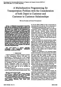
Definition 2.6. A UV  is called linear iff it has a linear UD. Symbolically: 0 , x  a   xa , a xb   x    ba 1, x  b  To indicate that  has a linear UD (Fig. 1), we shall write : L(a, b).

Fig. 1. Linear UD

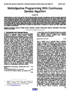
Fig. 2. Normal UD

Definition 2.7. A UV is called normal iff it has a normal UD. Symbolically: 1

    e  log x      x    1  exp    , x  0.1  3     To indicate that  has a normal UD (Fig. 2), we shall write  : N(e, ) .

Definition 2.8. An UV is called zigzag iff it has a zigzag UD. Symbolically:    0, x  a  x  a   x    , a xb  2 b  a   x  c  2b  , bxc  2  c  b 

To indicate that  has a zigzag UD (Fig. 3), we write : Z(a, b, c).


89

Fig. 3. Zigzag UD

Definition 2.9. Let ξ be a UV. The expected value of ξ is defined by 

0

E     M    r  dr 

 M    r  dr





0

provided that at least one of the two integrals is finite. It follows that E   



0

0



  1    r   dr     r  dr

3. Multiobjective geometric programming (MOGP) problem A multiobjective geometric programming (MOGP) problem can be written as

Find X   x1 , x2 , ..., xn 

T

(1)

So as to

Minimize f10  x  

p10

n

 x c10i

i 1

Minimize f 20  x  

k

k 10 i

k 1

p20

n

 x c20i

i 1

k

k 20 i

k 1

 Minimize f m 0  x  

pm 0

n

 x cm 0i

i 1

k

k 1

km 0 i


90

subject to fr  X  

pr

n

c x  ri

i 1

k

kri

 cr , r  1, 2, ..., q, xk > 0, k  1, 2, ..., n

k 1

where cj0i, are positive real numbers for all j = 1, 2, ..., m, i = 1, 2, ..., pr; kj0i and kri – real numbers for all k = 1, 2, ..., n, j = 1, 2, ..., m, i = 1, 2, ..., pr; pj0 – number of terms present in the j0th objective function, pr – number of terms present in the rth constraint, cr – boundary value for the rth constraint. In the above multiobjective non-linear programming model, there are m minimizing objective functions, q inequality type constraints and n strictly positive decision variables. In this section, we develop an MOGP model under uncertainty whose associated chance-constrained version admits an equivalent crisp formulation. First, we transform the conventional MOGP problem in Eq. (1) into an MOGP problem under uncertainty, where c j 0 i , cri , j = 1, 2, ..., m; i = 1, 2, ..., pr are UVs. The model is:

Find X   x1 , x2 , ..., xn 

T

(2)

So as to Minimize f10  x  

p10

n

 x c10i

i 1

Minimize f 20  x  

p20

k

k 10 i

k 1 n

 x c20i

i 1

k

k 20 i

k 1

 Minimize f m 0  x  

pm 0

n

 x i 1

cm 0i

k

km 0 i

k 1

subject to fr  X  

pr

n

 x  i 1

cri

k

kri

 cr r  1, 2, ..., q, k  1, 2, ..., n

k 1

where c j 0i – uncertain positive real numbers for all j = 1, 2, ..., m; i = 1, 2, ..., pr, c ri – uncertain boundary value for the rth constraint. In the above multiobjective non-linear geometric programming model, there are m minimizing objective functions, q inequality type constraints and n strictly positive decision variables.


91

Based on the model defined by Eq. (2) and the related constraints, we can formulate the following generic multiobjective GP model, which is a variant of the uncertain chance-constrained multiobjective geometric programming (UCCMOGP) model:

Find X   x1 , x2 , ..., xn 

T

(3)

So as to Minimize E  f10  x    Minimize E  f 20  x   

p10

n

c x 10 i

k

i 1

p20

k 10 i

k 1 n

 x c20i

i 1

k

k 20 i

k 1

 Minimize E  f m 0  x   

pm 0

n

c x m 0i

i 1

k

km 0 i

k 1

subject to  M ( f r  x)   M   

pr

n

c  x ri

i 1

k

k 1

kri

  cr    , r  1, 2, ..., q , xk  0, k  1, , ..., n,     

3.1. UCCMOGP model with linear uncertainty distributions

Let the coefficients c joi ,cri in Eq. (3) be independent positive linear UVs. That is to say,









a b c j 0 i : L c aj 0 i , c bj 0 i , with 0 < 0  c j 0i  c j 0i and cri : L cria , crib , with

0  cria  crib .

Lemma 3.1. Let i (i = 1, ..., n) be independent linear UVs, that is to say, i : L  ai , bi 

with ai < bi. Let Ui be non-negative variables. Then for every  M  

n



n

i 1



i 1

  0, 1 ,

U i  1        1    ai   bi  U i  1

Lemma 3.2. The expected value of a linear UV  : L a, bis E ( ab From Lemma 3.2, we obtain the following deterministic objective function for the UCCGP problem proposed in Eq. (3):


92

 E  

pj0

n

  c j 0i

i 1

 kj 0 i

xk

k 1

   

pj0

n





E (c j 0i )

i 1

pj0

 kj 0 i



xk

k 1

 i 1

 c aj 0i  cbj 0i   2 

   

n

x

 kj 0 i

k

, j  1, 2, ..., m

k 1

Moreover, from Lemma 3.1, the constraints in Eq. (3) admit the following equivalent deterministic form: 

pr



i 1

n



pr



i 1

i 1, ..., n, M  cri  xk kri  cr        k 1

n

  1    c a ri   c a ri   xk

kri

1

k 1

Thus, when the coefficients are UVs endowed with linear distributions, the model corresponding to Eq. (3) is equivalent to:

Find X   x1 , x2 , ..., xn 

T

(4)

So as to a b  c10  n k10i i  c10i   xk 2 i 1   k 1 p20 a b  c20i  c20i  n  k 20 i Minimize E  f 20  x      xk 2 i 1   k 1 

Minimize E  f10  x   

p10









Minimize E  f m 0  x   

 cma 0i  cmb 0i  2 i 1 

pm 0



  

n

x k

km 0 i

k 1

subject to: pr

 i 1

 1    cria   cria

n

 x

 kri

k

 1, r  1, 2, ..., q, xk  0, k  1, 2, ..., n,

  0, 1

k 1

Solution of MOGP problem by the weighted-sum method m   wj  1  be a set of non-negative weights. Using   j 1   the weighted sum technique, the above multiobjective model can be written as, n Let w j   w j : w   , w j  0,




Minimize E  f  x   

m





 w 

wj E f j 0  x  

j 1

pj0

m

j

j 1

i 1

 caj 0i  cbj 0i   2 

93

   

n

x

kj 0 i

k

k 1

Hence, the multiobjective optimization problem under uncertainty reduces to a single-objective crisp geometric programming problem as follows,

 c aj 0i  cbj 0i Minimize E  f  x    w j    2 j 1 i 1  pj0

m

 n   xk kj 0 i  k 1

5)

subject to pr

  1  c

a ri

  cria

i 1

n

 x

 kri

k

 1,

k 1

xk  0,    0, 1 , r  1, 2, ..., q, k  1, 2, ..., n Definition 3.1. A feasible solution x* is said to be a Pareto solution to the multiobjective programming problem under uncertainty (5), if there is no feasible solution x such that

 

 

E  f  x    E  f x*  , and E  f  x    E  f x*      for at least one index i. Definition 3.2. A feasible solution x* is said to be a weak Pareto solution to the multiobjective programming problem under uncertainty (5), if there is no solution x such that

 

E  f  x    E  f x*    Theorem 3.1. The solution of the MOGP problem (4), generated by the weighted sum method (5) is Pareto optimal if wj  0 for all j  1, 2, ..., m. Proof. Let x* be the solution of the MOGP problem (5), obtained by minimizing the m   m p j 0  caj 0i  cbj 0i  n kj 0i  xk . Obviously, it folfunction  f  x   w j E( f j 0  x    wj   k 1   j 1 i 1  2 j 1     lows that Ef  x *   E ( f  x  , x  X , which implies that



 




94 pj0

m

  wj

j 1



i 1

 caj 0i  cbj 0i   2  pj0

m

  wj

j 1

i 1

   

n



* xk kj 0i



k 1

 caj 0i  cbj 0i   2 

   

pj0

m

  wj

j 1

x n

kj 0 i

k

i 1

 caj 0i  cbj 0i   2 

* kj 0 i

 xk

k 1

   

n

x

kj 0 i

k

k 1

0

(6)

Suppose the solution x* of the problem (4) is not Pareto optimal. Then there exists some solution xʹ of the problem (4) satisfying Ef j 0  x    Ef j 0  x *  , which implies that Ef j 0

 x    Ef j 0

 x   0 for all *

j  1, 2, ..., m

pj0  c aj 0i  c bj 0i  n  c aj 0i  cbj 0i  n * kj 0 i   0 x  x       k 1 k kj 0i i 1   k 1 k 2 2 i 1     pj0  c aj 0i  c bj 0i  n  ( xk  xk* ) kj 0 i  0      2 i 1   k 1 By summing these inequalities and considering the assumption of the theorem that the weights w j are all positive, we obtain pj0









pj0

m

  wj

j 1

i 1

 c aj 0i  cbj 0i   2 



   



  x n

 kj 0 i

k

k 1

* kj 0 i

 xk

0

This inequality stands in contradiction to statement (6). Therefore, the solution x* is a Pareto solution for w j  0. Theorem 3.2. If x* is a Pareto-optimal solution of a convex multiobjective optimization problem, then there exists a non-zero positive weight vector w such that x* is a solution of the problem given by (5). For the proof, see Miettinen’s book on nonlinear multiobjective optimization [15]. 3.2. UCCMOGP model with normal uncertainty distributions

Let the coefficients c j 0i , cri in Eq. (3) be independent positive normal UVs, that is





to say, c j 0i : N c j 0i ,  j 0i , and cri : N  cri ,  ri , where c j 0i , cri ,  j 0i and  ri are all positive real values.


95

Lemma 3.3. Let i (i 1, ..., n) be independent normal UVs, that is to say,

i : N   i ,  i  where  I ,  i are all positive real values. Then for every    0, 1 ,  M  

n

 U i

i

i 1

 1   



n

   

i 1

i



i 3   log    1

   U i  1 

Lemma 3.4. The expected value of a normal UV  : Ne,  is E ( e From Lemma 3.4, we obtain the following deterministic objective function for the proposed UCCGP problem given by Eq. (3):

 E  

pj0

n

 x

 kj 0 i

c j 0i

i 1

k

k 1

   

pj0



n

x

 kj 0 i

E (c j 0i )

i 1

k

pj0



k 1

n

c x

 kj 0 i

j 0i

k

i 1

, j  1, 2, ..., m

k 1

Moreover, from Lemma 3.3, the constraints in Eq. (3) admit the following equivalent deterministic form: i 1, ..., n

 M  

pr

 xkkri  cr      k 1  n

  i 1

cri

pr

 i 1

  ri 3   log   cri    1 

   

n

x k

kri

1

k 1

Thus, when the coefficients are UVs endowed with normal distributions, the model corresponding to Eq. (3) is equivalent to: Find X   x1 , x2 , ..., xn 

T

(7)

So as to

Minimize E  f10  x    Minimize E  f 20  x   

p10

n

   c10i  xk i 1

k 1

p20

n

kj 10 i

   c20i  xk i 1

kj 20 i

k 1

 Minimize E  f m 0  x   

pm 0

n

   cm0i  xk i 1

k 1

kjm 0 i


96

subject to pr



  c i 1



ri



   

 ri 3   log    1

n

x k

kri

1

k 1

xk > 0, r  1, 2, ..., q, k  1, 2, ..., n,    0, 1 Solution of the MOGP problem by the weighted-sum method m   n Let w   w j : w   , w j  0, w j  1  be a set of non-negative weights. Using the   j 1   weighted sum technique, the above multiobjective model can be written as



pj0

m

Minimize

  wj

j 1

n

c j 0i

i 1

 x k

kj 0 i

k 1

Hence, this multiobjective optimization problem reduces to a single-objective crisp geometric programming problem as follows: pj0

m

Minimize

  wj

j 1

n

c j 0i

i 1

 x k

kj 0 i

(8)

k 1

subject to pr

 i 1

  ri 3   log   cri    1 

   

n

x k

kri

1

k 1

xk > 0, r  1, 2, ..., q, k  1, 2, ..., n,    0, 1 3.3. UCCMOGP model with zigzag uncertainty distributions

c , c Let the coefficients j 0i ri in Eq. (3) be independent positive zigzag UVs. That is to say, c j 0i : Z (c aj 0i , c bj 0i , c aj 0i ), with 0 < c aj 0i , cbj 0i , c aj 0i and cri : Z (c aj 0i , c bj 0i , c aj 0i ), with 0 < c aj 0i , cbj 0i , c aj 0i (Fig. 3). Lemma 3.5. Let i (i 1, ..., n) be independent zigzag UVs, that is to say,

i : Z  ai , bi , ci  with ai  bi  ci . Let Ui be non-negative variables. Then for every

   0, 1


97

 n if    0, 0.5    1  2  ai  2 bi  U i  1,   n    i 1 M  iU i  1       i 1   n   2  1  ci  2  1    bi  U i  1, if    0.5, 1   i 1







Lemma 3.6. The expected value of a zigzag UV  : Z(a, b, c) is E ( ) a + 2b + c)/4) From Lemma 3.6, we obtain the following deterministic objective function for the proposed UCCGP problem given by Eq. (3):  pj0 E  c j 0i  i 1

n

 

 kj 0 i

xk

k 1

  

pj0

n





E (c j 0i )

i 1

 kj 0 i

xk

pj0



k 1



c aj 0i  2c bj 0i  c cj 0i 4

i 1

n

x

 kj 0 i

k

, j  1, 2, ..., m

k 1

Moreover, from Lemma 3.5, the constraints in Eq. (3) admit the following equivalent deterministic form: i 1, ..., n  M   

pr

 xk kri  cr   k 1  n

  i 1

cri

pr n  xxk kri  1, if    0, 0.5   1  2  cria  2 crib   i 1 k 1    n  pr xk kri  1, if    0.5, 1  2  1  cric  2  1    cb ri  k 1  i 1









Thus, when the coefficients are UVs endowed with zigzag distributions, the model corresponding to Eq. (3) is equivalent to: For  < 0.5 we have Find X   x1 , x2 , ..., xn 

T

(9)

So as to p10

Minimize E

a b c  c10  i  2c10 i  c10 i  4  

 f10  x      i 1

n

x k

k 1

k 10 i


98

a b c  c20 i  2c20i  c20i Minimize E  f 20  x     4 i 1   p20



Minimize E  f m0  x   

  

n

x k

k 20 i

k 1

 cma 0i  2cmb 0i  cmc 0i  4 i 1 

  

pm 0



n

x k

km 0 i

k 1

subject to pr

n

   1  2  cria  2 crib  xk i 1

kri

1

k 1

  0, 1

xk > 0, r  1, 2, ..., q, k  1, 2, ..., n, For  > 0.5 we have

Find X   x1 , x2 , ..., xn 

T

(10)

so as to a b c  c10  n k 10 i i  2c10i  c10i   xk 4 i 1   k 1 p20 a b c  c20i  2c20i  c20i  n k 20 i Minimize E  f 20  x      xk 4 i 1   k 1 

Minimize E  f10  x   

p10









Minimize E  f m0  x   

 cma 0i  2cmb 0i  cmc 0i  4 i 1 

pm 0



  

n

x k

km 0 i

k 1

subject to pr

   2  1  c

c ri

 2  1    crib

i 1

n

 x

 kri

k

1

k 1

xk > 0, r  1, 2, ..., q, k  1, 2, ..., n,

  0, 1

Solution of the MOGP problem by the weighted-sum method

Let w  ( w j : w   n , w j  0,

m

w

j

 1) be a set of non-negative weights. Using the

j 1

weighted sum technique, the above multiobjective model can be written as,

Multiobjective geometric programming problem under uncertainty pj0

m

Minimize

  wj

j 1

i 1

 caj 0i  2cbj 0i  ccj 0i   4 

   

n

99

x

kj 0 i

k

k 1

Hence, this multiobjective optimization problem under uncertainty reduces to a single-objective crisp geometric programming problem: For  < 0.5 we have pj0

m

Minimize

  wj

j 1

i 1

 caj 0i  2cbj 0i  ccj 0i   4 

   

n

x

kj 0 i

k

(11)

k 1

subject to pr

   1  2 

cria

 2

crib

i 1

n

 x

 kri

1

k

k 1

xk > 0, r  1, 2, ..., q, k  1, 2, ..., n,

  0, 1

For  > 0.5 we have

Minimize

i 1

 caj 0i  2cbj 0i  ccj 0i   4 

cric

  1  2 

pj0

m

w  j

j 1

   

n

x

 kj 0 i

k

(12)

k 1

subject to pr

   2  1  i 1

crib

n

 x

k

 kri

1

k 1

xk > 0, r  1, 2, ..., q, k  1, 2, ..., n,

  0, 1

4. Numerical examples Optimization is the process of finding the point that minimizes an appropriately defined function. More specifically:  A local minimum of a function is a point where the value of the function is smaller than or equal to the value at nearby points, but possibly greater than at a distant point.  A global minimum is a point where the value of a function is smaller than or equal to the value at all other feasible points (the numerical examples which are given here give the global optimal).


100

Fig. 4. Local and global minima

We now give some numerical examples to show the efficacy of the MOGP models.  min f10  x   c 101  c102x2 x3 x1 x2 x3

min f 20  x  

(13)

c 201 such that c 11x1 x2  c 12x1 x3  4, x1 , x2 , x3  0 x1 x2 x3

4.1. Example for linear uncertainty distributions c101 : L  30, 50  , c102 : L  30, 50  , c201 : L  700, 900  , c11 : L  0.8, 1.2  , c12 : L  1.6, 2.4 

Thus the UCCMOGP problem is

min f10  x  

40  40 x2 x3 x1 x2 x3

(14)

800 min f 20  x   x1 x2 x3 such that

 0.8  1     1.2  x1x2   1.6  1     2.4  x1x3  4,

x1 , x2 , x3  0

From Eq. (5), the problem given by Eq. (14) becomes the following deterministic weighted-sum MOGP:

min f



 40w1  800w2 40 800  40 x2 x3   w2   40w1 x2 x3 (15) x1 x2 x3 x1 x2 x3  x1 x2 x3 

 x   w1 


101

such that

 0.8  1     1.2  x1x2   1.6  1     2.4  x1x3  4,

x1 , x2 , x3  0

 4   3  1  0.

Here, DD The dual multiobjective geometric programming problem (DMOGPP) corresponding to (15) is  01

 40w1  800w2  max d        01  

 02

 40w1      02 



  0.8  1     1.2   11     411  



  01.6  1     2.4   12        11  12  11 12   412   such that

01  02  1,  01  11  12  0,  01   02  11  0  01   02  12  0, w1  w2  1,  01 ,  02 , 11 , 12  0 Solving the above normal and orthogonal conditions, we have

2 3

1 3

1 3

01  , 02  , 11  , 12 

1 3

From the primal-dual relation, we obtain 40 w1  800 w2   01d    , 40 w1 x2 x3   02 d   x1 x2 x3

 0.8  1     1.2  x1x2  4

11 , 11  12



 1.6  1     2.4  x1x3  4

12 11  12

and the corresponding optimal solution is  w1  20 w2 x3    4  1.6  1     2.4 ) w1 

1/3

   

, x2  2 x3 , x1 

2  1.6  1     2.4 )  x3


102

Table 1. Optimal solution under linear UDs



0.2

0.4

0.6

0.8

Weight w1

w2

0.1 0.5 0.9 0.1 0.5 0.9 0.1 0.5 0.9 0.1 0.5 0.9

0.9 0.5 0.1 0.9 0.5 0.1 0.9 0.5 0.1 0.9 0.5 0.1

Optimal values Primal variables Objective functions x1* x2* x3* f 01* ( x) f 02* ( x) 0.38 0.79 1.48 0.36 0.74 1.39 0.34 0.71 1.32 0.33 0.67 1.26

5.90 2.88 1.54 5.74 2.80 1.50 5.58 2.72 1.46 5.44 2.66 1.42

2.95 1.44 0.77 2.87 1.40 0.75 2.79 1.36 0.73 2.72 1.33 0.71

702.25 178.10 70.22 665.70 170.59 70.58 630.28 163.20 71.06 600.06 158.39 71.82

120.96 244.18 455.84 134.90 275.79 511.59 151.14 304.60 568.64 163.84 337.51 629.76

4.2. Example for normal uncertainty distributions

c101 : N  40,4 , c102 : N  40,4 , c201 : N  800,80 , c11 : N 1,0.1 , c12 : N  2,0.2 . Then the UCCMOGP problem is

min f10  x  

40  40 x2 x3 x1 x2 x3

(16)

800 min f 20  x   x1 x2 x3 subject to  0.1 3   log   1   1 

 0.2 3    log    x1 x2   2    1 

   x1 x3  4 

From Eq. (8), the problem given by Eq. (16) becomes the following deterministic weighted-sum MOGP:

 40  40w1  800w2 800  40 x2 x3   w2   40w1 x2 x3 Min f  x   w1  x1 x2 x3 x1 x2 x3  x1 x2 x3  such that

(17)


 0.1 3   log   1   1 

 0.2 3    log    x1 x2   2    1 

103

   x1 x3  4, x1 , x2 , x3  0 

Here, DD = 4 – (3 + 1) = 0. The DMOGPP corresponding to (17) is   0.1 3   log  1   01  02     40 w1  800 w2   40 w1    1 max d         411  01     02    0.2 3   log    2   1    412 

        

        

11

12

11  12 

11 12 

such that

01  02  1,  01  11  12  0,  01  02  11  0 01  02  12  0, w1  w2  1, 01 , 02 , 11, 12  0 Solving the above normal and orthogonal conditions, we have

2 3

1 3

1 3

01  , 02  , 11  , 12 

1 3

From the primal-dual relation, we obtain 40 w1  800 w2   01d   , 40 w1 x2 x3   02 d   x1 x2 x3

 0.1 3   log   1   1  4

   x1 x2 

 0.2 3   log   2   1 11 ,   11  12 4

   x1 x3 



12 11  12

and the corresponding optimal solution is 1/3

w1  20w2 2   x3   , x2  2 x3 , x1    0.2 3     4  2  0.2 3 log     w  2 log   1     x3        1       1       


104

Table 2. Optimal solution under normal UDs



0.2

0.4

0.6

0.8

Weight w1

w2

0.1 0.5 0.9 0.1 0.5 0.9 0.1 0.5 0.9 0.1 0.5 0.9

0.9 0.5 0.1 0.9 0.5 0.1 0.9 0.5 0.1 0.9 0.5 0.1


5.80 2.84 1.52 5.70 2.78 1.48 5.62 2.74 1.46 5.52 2.70 1.44

2.90 1.42 0.76 2.85 1.39 0.74 2.81 1.37 0.73 2.76 1.35 0.72

679.23 174.36 70.59 656.28 167.84 68.49 638.18 163.64 67.99 616.14 159.52 67.19

128.55 261.02 487.69 129.59 265.42 500.32 129.89 269.77 507.17 134.64 274.35 514.40

4.3. Example for zigzag uncertainty distributions c101 : Z  30, 40, 60  , c102 : Z  30, 40, 50  , c201 : Z  700,800,1000  c11 : Z  0.8,1.0,1.2  , c12 : Z 1.6, 2.2.4  .

For  < 0.5 we have: The UCCMOGP problem is

min f10  x  

42.5  40 x2 x3 x1 x2 x3

(18)

825 min f 20  x   x1 x2 x3 subject to

 0.8 1  2   1.0  2   x x  1.6 1  2   2.0  2   x x 1 2

1 3

 4, x1 , x2 , x3  0

From Eq. (11), the problem given by Eq. (18) becomes the following deterministic weighted-sum MOGP:  42.5  825 42.5w1  825w2 min f  x   w1   40 x2 x3   w2   40 w1 x2 x3 x1 x2 x3 x1 x2 x3  x1 x2 x3 

(19)


105

such that

 0.8 1  2   1.0  2   x x  1.6 1  2   2.0  2   x x 1 2

1 3

 4, x1 , x2 , x3  0

Here, DD = 4 – (3 + 1) = 0. The DMOGPP corresponding to (19) is  01

 02

 42.5w1  825w2   40 w1  max d         01     02 

  01.6 1  2   2.0  2        412  

  0.8 1  2   1.0  2        411  

11

12

11  12 

11 12 

such that

01  02  1,  01  11  12  0,  01  02  11  0 01  02  12  0, w1  w2  1, 01 , 02 , 11, 12  0 Solving the above normal and orthogonal conditions, we have

2 3

1 3

1 3

01  , 02  , 11  , 12 

1 3

From the primal-dual relation, we obtain 42.5 w1  825 w2   01d   , 40 w1 x2 x3   02 d   x1 x2 x3

0.8 1  2   1.0  2  4



1.6 1  2   2.0  2  11 12 ,  11  12 11  12 4

and the corresponding optimal solution is, 1 /3

42.5 w1  825 w2     2 40 x3    , x2  2 x3 , x1  1.6 1  2   2.0  2   x3  4 1.6 1  2   2.0  2   w1   


106

For  > 0.5, we have: The UCCMOGP problem is

min f10  x  

42.5  40 x2 x3 x1 x2 x3

(20)

825 min f 20  x   x1 x2 x3 such that

1.2  2  1  2 1   1.0 x x   2.4  2  1  2 1    2.0 x x 1 2

1 3

 4, x1 , x2 , x3  0

From Eq. (12), the problem given by Eq. (20) becomes the following deterministic weighted-sum MOGP:  42.5  825 42.5w1  825w2 min f  x   w1   40 x2 x3   w2   40w1 x2 x3 x1 x2 x3 x1 x2 x3  x1 x2 x3 

(21)

such that

1.2  2  1  2 1   1.0 x x   2.4  2  1  2 1    2.0 x x 1 2

1 3

 4, x1 , x2 , x3  0

Here, DD = 4 – (3 + 1) = 0. The DMOGPP corresponding to (21) is  01

 42.5w1  825w2   40 w1  max d         01     02 

 02

 1.2  2  1  2 1   1.0       411  

  2.4  2  1)   2 1    2.0       4  12  

12

11  12 

11 12 

such that

01  02  1,  01  11  12  0,  01  02  11  0 01  02  12  0, w1  w2  1, 01 , 02 , 11, 12  0

11


Solving the above normal and orthogonal conditions, we have

2 3

1 3

1 3

01  , 02  , 11  , 12 

1 3

From the primal-dual relation, we obtain

42.5w1  825w2   01d   , 40 w1 x2 x3   02 d   x1 x2 x3

1.2  2  1  2 1   1.0 4



2.4  2  1  2 1    2.0 11 12 ,  , 11  12 11  12 4

and the corresponding optimal solution is, 1/3

42.5w1  825w2     40 x3    , x2  2 x3  4  2.4  2  1  2 1    2.0  w1    2 x1   2.4  2  1  2 1    2.0  x3 Table 3. Optimal solution under zigzag UDs



0.2

0.4

0.6

0.8

Weight w1

w2

0.1 0.5 0.9 0.1 0.5 0.9 0.1 0.5 0.9 0.1 0.5 0.9

0.9 0.5 0.1 0.9 0.5 0.1 0.9 0.5 0.1 0.9 0.5 0.1


5.96 2.90 1.56 5.80 2.82 1.52 5.64 2.76 1.48 5.50 2.68 1.44

2.98 1.45 0.78 2.90 1.41 0.76 2.82 1.38 0.74 2.75 1.34 0.72

716.73 181.16 72.60 679.82 173.49 73.06 644.05 168.29 73.66 613.03 160.08 69.94

122.24 251.53 464.39 136.25 280.38 521.29 152.56 309.43 579.45 155.84 319.07 552.58

107

108


5. Conclusions Multiobjective geometric programming (MOGP) is a powerful optimization technique widely used for solving a variety of nonlinear optimization problems, particularly in engineering. Conventional MOGP models assume that the parameters are deterministic and crisp. However, the parameters or coefficients in real-life MOGP problems are often imprecise and subject to fluctuations. Therefore, we have approached the problem of formalizing and implementing imprecise and non-deterministic parameters using uncertainty theory. There exists an ample literature on MOGP under uncertainty and its applications to problems (either chance-constrained or not) whose coefficients are fuzzy numbers, fuzzy variables or random variables. However, to the best of our knowledge, no previous study has dealt with the formulation and/or solution of MOGP problems where the coefficients are given by uncertain variables (UVs). In this paper, we have introduced an uncertain chance-constrained multiobjective GP (UCCMOGP) model and proposed a method of solution that applies to three of the most commonly used uncertainty distributions: we assumed the coefficients to be uncertain variables with linear, normal or zigzag uncertainty distributions. We proved that the corresponding uncertain chance-constrained multiobjective geometric programming (UCCMOGP) models can be transformed into conventional multiobjective geometric programming (MOGP) problems with crisp coefficients and, hence, an optimal solution can be found using the duality algorithm. We have shown the efficacy of the proposed model through three numerical examples. We believe that the framework proposed in this paper contributes to shedding light on the applications of MOGP to concrete problems, opening the way to further research in engineering and production management. References [1] BEIGHTLER C.S., PHILIPS D.T., Foundation of optimization, Prentice-Hall, New Jersey 1979. [2] BISHAL M.P., Fuzzy programming technique to solve multiobjective geometric programming problems, Fuzzy Sets Syst., 1992, 51, 67–71. [3] CHANGKONG V., HAIMES Y.Y., Multiobjective Decision Making, North-Holland, New York 1983. [4] DAS P., ROY K.T., Multiobjective geometric programming and application in gravel box problem, J. Global Res. Comp. Sci., 2014, 5 (7), 6–11. [5] DING S., The α-maximum flow model with uncertain capacities, Appl. Math. Model., 2015, 39 (7), 2056–2063. [6] DUFFIN R.J., PETERSON E.L., ZENER C., Geometric Programming. Theory and Application, Wiley, New York 1967. [7] HAN S., PENG Z., WANG S., The maximum flow problem of uncertain network, Inform. Sci., 2014, 265, 167–175. [8] ISLAM S., ROY T.K., Multiobjective marketing planning inventory model. A geometric programming approach, Appl. Math. Comp., 2008, 205 (1), 238–246. [9] LI S., PENG J., ZHANG B., The uncertain premium principle based on the distortion function, Insur. Math. Econ., 2013, 53, 317–324.


109

[10] LIU B., Some research problems in uncertainty theory, J. Uncertain Syst., 2009, 3 (1), 3–10. [11] LIU B., Uncertain risk analysis and uncertain reliability analysis, J. Uncertain Syst., 2010, 4 (3), 163–170. [12] LIU B., Uncertain set theory and uncertain inference rule with application to uncertain control, J. Uncertain Syst., 2010, 4 (2), 83–98. [13] LIU B., Uncertainty Theory, 4th Ed., Springer-Verlag, Berlin 2015. [14] LIU G.P., YANG J.B., WHIDBORNE J.F., Multiobjective optimization control, Research Studies Press Ltd., Hertfordshire 2003. [15] MIETTINEN K.M., Non-linear multiobjective optimization, Kluwer’s Academic Publishing, 1999. [16] OJHA A.K., DAS A.K., Multiobjective geometric programming problem being cost coefficients as continuous function with mean method, J. Comp., 2010, 2 (2), 67–73. [17] OJHA A.K., BISWAS K.K., Multiobjective geometric programming problem with ε-constraint method, Appl. Math. Model., 2014, 38 (2), 747–758. [18] OJHA A.K., OTA R.R., Multiobjective geometric programming problem with Karush–Kuhn–Tucker condition using -constraint method, RAIRO-Oper. Res., 2014, 48, 429–453. [19] PENG J., YAO K., A new option pricing model for stocks in uncertainty markets, Int. J. Oper. Res., 2011, 8 (2), 18–26. [20] SHIRAZ R.K., TAVANA M., DI CAPRIO D., FUKUYAMA H., Solving geometric programming problems with normal, linear and zigzag uncertainty distributions, J. Opt., Theory Appl., 2016, 170 (1), 243–265. [21] SHIRAZ R.K., TAVANA M., FUKUYAMA H., DI CAPRIO D., Fuzzy chance-constrained geometric programming. The possibility, necessity and credibility approaches, Oper. Res., 2017, 17 (1), 67–97. [22] WANG X.S., GAO Z.C., GUO H.Y., Delphi method for estimating uncertainty distributions, Information, 2012, 15 (2), 449–460. [23] WANG X.S., GAO Z.C., GUO H.Y., Uncertain hypothesis testing for expert’s empirical data, Math. Comput. Model., 2012, 55 (3–4), 1478–1482. [24] WORRALL B.M., HALL M.A., The analysis of an inventory control model using posynomial geometric programming, Int. J. Prod. Res., 1982, 20, 657–667. [25] YANG H.H., BRICKER D.L., Investigation of path-following algorithms for signomial geometric programming problems, Eur. J. Oper. Res., 1997, 103, 230–241. [26] ZHU J., KORTANEK K.O., HUANG S., Controlled dual perturbations for central path trajectories in geometric programming, Eur. J. Oper. Res., 1992, 73, 524–531. [27] ZHU Y., Uncertain optimal control with application to a portfolio selection model, Cybernet. Syst., 2010, 41 (7), 535– 547. Received 27 June 2017 Accepted 6 December 2017