A Modified Bayesian Method (MBM) for estimating directional wave spectra from Doppler ..... u is a type of weighting coefficient which represents the smoothness of X , .... Eq. (29) is not valid for the lower limit(. )1 i = and the upper limit. (. ) i M. = ..... Position of HF ocean radar systems at Master and Slave (UK) and the wave ...
VERIFICATION OF A MODIFIED BAYESIAN METHOD FOR ESTIMATING DIRECTIONAL WAVE SPECTRA FROM HF RADAR Lukijanto 1, Noriaki Hashimoto 2 and Masaru Yamashiro 3 A Modified Bayesian Method (MBM) for estimating directional wave spectra from Doppler spectra obtained by HF radar is examined using field data which were employed in the verification of Bayesian Method (BM). Applicability, validity and accuracy of the MBM are demonstrated compared with the directional wave spectra estimated by BM and observed by buoy acquired from the reliable field data obtained from Surface Current and Wave Variability Experiments (SCAWVEX) project. The necessary conditions of the Doppler spectral components to be used to estimate a reliable directional spectrum are correspondingly estimated by BM. The results clearly demonstrate that directional wave spectra can be estimated by MBM on the basis of Doppler spectra. In addition, though BM shows very time consuming in computations, BM is more robust against the presence of noise than MBM. Keywords: HF radar; directional wave spectrum; spectrum; wave observation; wave data analysis; currents measurement; Bayesian method
1.
Introduction
The measurement of directional wave spectra is important for wave research and solving many ocean and coastal engineering problems. The high frequency (HF) radar has offered the ability to measure directional wave spectra since Crombie (1955) observed and identified the distinctive features of Doppler spectra. Barrick (1972) derived the exact theoretical formulation that expressed the Doppler spectra in terms of directional wave spectra and the surface current velocity. To estimate directional wave spectra from HF radar data, it is necessary to solve a complicated two-dimensional nonlinear integral equation. Studies on this matter have been developed on the basis of theoretical aspects, and still include one of the greatest barriers to accurately estimate Doppler spectra. The methods for estimating directional wave spectra from Doppler spectra obtained by High Frequency (HF) radar backscatter remain unexplored compared to the ones for estimating ocean surface currents. The Bayesian Method developed by Hashimoto and Tokuda (1999) has shown as an accurate and reliable method among other existing methods, e.g. Wyatt (1990), Howel and Walsh (1993) and Hisaki (1996), for estimating directional wave spectra from Doppler spectra. A Bayesian Method was examined by the numerical simulation and actual field data obtained during the Surface Current and Wave Variability Experiments (SCAWVEX) project (Hashimoto et al, 2003). However, this method is still at the theoretical level and has not been put into practical use yet because of its drawbacks of time consuming computation and large memory size requirements. For these reasons, a practical method for estimating directional wave spectra from Doppler Spectra is principally required to estimate directional wave spectrum efficiently. This sophisticated method, namely Modified Bayesian Method, has been developed by retaining to the advantages of Bayesian Method and introducing a similar formulation of Maximum Entropy Principle (Hashimoto and Kobune, 1986). A proposed mathematical formulation of the directional wave spectrum in the Modified Bayesian Method is assumed as an exponential function having the power expressed by a Fourier series over the direction and piecewise constant function over the frequency (Lukijanto et al, 2009a). Indeed, Modified Bayesian Method has been more efficient than Bayesian Method since the developed method is capable of executing high speed computations and reducing the memory usage. Subsequently, the validity and accuracy of the developed method is necessary to be examined further to the actual Doppler spectra. In this study, we apply the Modified Bayesian Method proposed by Lukijanto et al (2009a) to some of the above-mentioned SCAWVEX data, from which some reliable estimated directional wave spectra are reported. We verify the applicability and accuracy of the Modified Bayesian Method and discuss some results on further improvements of the developed method for the future practical use in the operational wave measurements. The necessary conditions of the Doppler spectral components to be used to estimate a reliable directional spectrum are correspondingly estimated by Bayesian Method as reported detail in Hashimoto et al (2003).
1 2 3
PTISDA-BPPT, Jl.MH. Thamrin 8, Jakarta 10340, Indonesia Dept. of Urban and Environmental Eng., Kyushu University, Motooka 744, Nishi-ku, Fukuoka, 819-0395, Japan Dept. of Urban and Environmental Eng., Kyushu University, Motooka 744, Nishi-ku, Fukuoka, 819-0395, Japan
1
2 2.
A Bayesian Method
The ocean surface waves consist of various component waves with different frequency and propagation direction. The Doppler spectrum, σ (ω ) , obtained by HF radar represents the energy distribution of the radio wave signal backscattered by the ocean surface waves at the angular frequency ω , and is expressed by the summation of the first-order component, σ (1) (ω ) , and the second-order component, σ (2) (ω ), i.e. σ (ω ) ≈ σ (1) (ω ) + σ (2) (ω ). The relationship between the Doppler spectra and directional wave spectra is mathematically expressed by the following equations for deep water conditions (Barrick, 1972):
σ (1) (ω ) = 26 π k04 ∑ S (−2mk0 , 0) δ (ω − mωB )
(1)
m = ±1
= σ (2) (ω ) 26 π k04
∑ ∫∫
m1 , m2 = ±1
∞
−∞
| Γ |2 S (m1k1 ) S (m2 k 2 )
(2)
× δ (ω − m1 gk1 − m2 gk2 ) dpdq
where k0 = (k0 , 0) is the absolute value of the wave number vector k 0 of radio waves,
S (k ) = S (k x , k y ) is the wave number spectrum of ocean surface waves and ωB (= 2gk0 ) is the Bragg angular frequency. The independent variables, p and q, of the integration represent coordinates, each of which is parallel to the axis of the radar beam and orthogonal to the radar beam respectively. The wave number vectors for ocean waves, k1 and k 2 , are related to these variables by the following equations: k1 =( p − k0 , q ), k 2 =(− p − k0 , − q )
(3)
These relations indicate the Bragg’s resonance condition expressed by k1 + k 2 = −2k 0
(4)
The coupling coefficient, Γ , shows the degree of the contribution from the wave components having the wave number k1 and k 2 to the second-order energy distribution of the backscattered radar signal, and commonly expressed by Γ = Γ E + Γ H (Barrick, 1972), the summation of the electromagnetic scattering effect, Γ E , and the hydrodynamic scattering effect, Γ H . Since the first-order component σ (1) (ω ) and the second-order component σ (2) (ω ) appear in different frequencies in the Doppler spectrum σ (ω ) , they can be separated; even though they are small in magnitude. Consequently, valuable oceanographic information such as surface currents and waves can be obtained from the respective spectrum components. As shown in Eq. (2), the two component waves having the wave number vector k1 and k 2 are related to the second-order component σ (2) (ω ). This means that Eq. (2) includes the contributions of an infinite numbers of component waves having different frequency ω and propagation direction θ , and hence in principle, the directional spectrum can be estimated based on this information. When the directional spectrum is estimated based on Eq. (2), the following problems arise: 1)
2)
Due to the constraint of the δ function, the integration of Eq. (2) must be executed along a curve on the “frequency direction” plane into which the wave number plane is transformed by the dispersion relationship. The digitization of the integral of Eq. (2) is therefore complicated. This is a so-called incomplete inverse problem in which the number of unknown parameters is much larger than that of equations obtained from the measurements. This sometimes causes the problem that even a small measurement error would seriously deteriorate the reliability of the estimate.
3 To estimate directional spectrum from HF radar data, it is necessary to solve a complicated twodimensional nonlinear integral Eq. (2). Since Eq. (2) includes the contributions of infinite numbers of component waves having different frequencies ω and propagation directions θ ; thus we will focus on the second-order scattering component σ (2) (ω ) and introduce a method for estimating directional wave spectra from this second-order scattering component. In this study, deep water waves have been examined. Besides, the method developed for deep water waves can be easily extended to shallow water waves. For mathematical convenience, the parameters are non dimensionalized by the Bragg angular frequency, ωB , and the doubled wave number of the radio wave, 2k0 , as follows:
ω ω= / ωB = k k /(2k0 ) Γ = Γ /(2k ), S (k ) = (2k ) 4 S (k ) 0 0
(5)
The integration of the second-order component Eq. (2) with respect to the two variables p and q axis can be transformed into a single variable since the integrand includes the delta function δ . If the wave propagation direction θ1 of the wave number vector k1 is adopted as a single independent variable for the integration, Eq. (2) can be transformed as follows (Lipa and Barrick, 1982): θL
σ (2) (ω ) = ∫ G (θ1 , ω )dθ1
(6)
0
where
{
(θ , ω ) 16π | Γ |2 S (m1k 1 ) S (m2 k 2 ) G= + S (m1k 1 *) S (m2 k 2 *) y 3 dy / dh y = yˆ
}
dy = dh
y ( y 2 + cos θ1 ) 1 + m1m2 4 ( y + 2 y 2 cos θ1 + 1)3 / 4
(7)
−1
(8)
and y = k1 . yˆ can be obtained by solving Eq. (9).
ω − m1 yˆˆˆ− m2 ( y 4 + 2 y 2 cos θ1 + 1)1/ 4 = 0
(9)
k i * is the nondimensional symmetry wave number vector of k i with respect to the radar beam axis (the p − axis ). An upper limit of integration can be given by θ L = π when ω ≤ 2, and θ L= π − cos −1 (2 / ω 2 ) when ω > 2 , respectively. The wave number spectrum S (k ) in Eq. (7) can be transformed into the frequency-direction spectrum (directional wave spectrum) S ( f , θ ) as follows: g2 S (k ) = 5 4 3 S ( f , θ ) (10) 2π f Thus, by imposing the directional wave spectrum S ( f , θ ) , the second-order component σ (2) (ω ) measured by the HF radar can be theoretically calculated by numerical integration of Eq. (6). In the original Bayesian Method (Hashimoto and Tokuda, 1999), directional spectrum is treated as a piecewise constant function with respect to each energy component of frequency and direction, including M × N unknown parameters. Here, M is the number of frequency segments, while N is the number of direction segments. The problem for estimating directional wave spectrum with HF radar is to estimate a non-negative solution of S ( f , θ ) based on simultaneous integral equations of Eq. (6) set up for σ (2) (ω ) . Although, generally the directional wave spectrum is S ( f , θ ) ≥ 0 , in this study, it is
4 treated as S ( f , θ ) > 0 , and assumed to be exponential piecewise constant function over the directional range from 0 to 2π and the frequency range from f min to f max (Hashimoto, 1987). In addition, this assumption is commonly employed in numerically generating random waves. M
N
S ( f , θ ) = α ∑∑ exp ( xi , j ) δ i , j ( f , θ )
(11)
=i 1 =j 1
where xi , j = ln{S ( f i , θ j ) / α } , M is the number of segments ∆f of frequency f , while I is the number of segments ∆θ of direction θ , and
1 : fi −1 ≤ f < fi and θ j −1 ≤ θ < θ j
δi, j ( f ,θ ) =
0 : otherwise
(12)
α is a parameter introduced to normalize the magnitude of xi , j , and given by 2π
∫ ∫ S ( f ,θ ) dfdθ α= ∫ ∫ dfdθ f max
f min
0
f max
f min
(13)
2π
0
The numerator on the right hand side of Eq. (13) is approximately given by the following equation (Barick, 1977): ∞
∫ ∫ f max
f min
2π
0
S ( f , θ ) dfdθ ≈
2 ∫ {σ ( 2) (ω ) / W (ω / ω B )}d ω −∞
∞
k02 ∫ σ (1) (ω ) d ω
(14)
−∞
) 8 | Γ 2 | / k02 is a weighting function and Γ is an approximate coupling coefficient of where W (ω / ωB= Γ (Barick, 1977). The frequency f and the direction θ are discretized by the following equations respectively. = µi ln = f i ln f i −1 + ∆f , θ= θ j −1 + ∆θ j
(15)
Substituting Eq. (11) into Eq. (6) yields an integral equation including unknown variables M × N . After digitizing the Eq. (6) by replacing the integration with the summation Σ , the integral equation can be approximated by the nonlinear algebraic equation. However, it is unrealistic to assume that the energy distribution over wave frequency f and wave propagation direction θ can be discontinuous. Thus, S ( f , θ ) is generally considered to be a continuous and smooth function. The integral of Eq. (6) is, however, a curvilinear integral where the integration must be performed along a special path in ( f , θ ) plane due to the restrictions of Eqs. (4) and (9). As mentioned earlier, Eq. (6) includes a singular point, and has to be integrated with smaller segments around the singular point. In discretizing Eq. (6), the value of the directional wave spectrum along the path in ( f , θ ) plane is linearly interpolated by the neighboring grid point values of the directional wave spectrum in the same way as Hisaki (1996), and expressed by
S ( µ ,θ ) = (1 − ξ ) S ( µi , θ ) + ξ S ( µi +1 , θ ) + (1 − ξ ) ζ S ( µi , θ j +1 ) + ξ ζ S ( µi +1 , θ j +1 )
(16)
where µ = ln f , 0 ≤ ξ and ζ ≤ 1 . Eq. (6) can therefore be digitized with respect to the grid point values of S ( µi , θ j ) with the desired degree of accuracy.
5 Finally, by taking into account the errors ε k of the Doppler spectrum, the integral Eq. (6) can be approximated by the nonlinear algebraic equation including the unknown X = ( x1, 1 , , xI , J )t , and expressed by:
= σ k(2) Fk ( X) + ε k
(17)
where the suffix k indicates a value of the Doppler frequency ω k (k = 1, , K ) . The errors ε k (k = 1, , K ) of every Doppler frequency ω k are assumed to be independent of each other and their occurrence probabilities can be expressed by a normal distribution having a zero mean and variance λ 2 . Then, for a given σ k(2) (k = 1, , K ) , the likelihood functions of X and λ 2 is given by: L( X; λ 2 ) =
1 exp − 2 K ( 2π λ ) 2λ 1
∑{ σ K
(2) k
}
− Fk ( X)
k =1
2
(18)
It should be noted that the directional wave spectrum S ( f , θ ) has thus far been expressed by a piecewise constant function, with the correlation between the wave energy of each segment of ∆f × ∆θ not yet having been taken into account. As directional wave analysis is commonly based on the linear wave theory, it can be assumed that each of energy on each segment is independent of each other. In general, S ( f , θ ) is considered to be a continuous and smooth function. This allows an introduction of an additional condition that the local variation of = xi , j (i 1,= , I ; j 1, , J ) can be well approximated by a smooth surface so that the value given in Eq. (19) is expected to be small. xi , j +1 + xi +1, j + xi , j −1 + xi −1, j − 4 xi , j
(19)
In the upper boundary ( i = I ) and the lower boundary ( i = 1 ) of the frequency f , the value given in Eq. (20) is expected to be small as a priori condition. xi , j +1 − 2 xi , j + xi , j −1
(20)
These additional conditions lead to I −1
∑∑ ( x
i , j +1
i =2
j
+
∑
+ xi +1, j + xi , j −1 + xi −1, j − 4 xi , j ) 2 2
( x1, j +1 − 2 x1, j + x1, j −1 ) +
j
∑
( xI , j +1 − 2 xI , j + xI , j −1 )
2
(21)
→ small
j
(where xi ,0 = xi , J , xi , −1 = xi , J −1 ) From algebraic viewpoint, Eq. (21) can be written in the matrix form, as || DX ||2
(22)
where D is the coefficient matrix of Eq. (21). It is, therefore, surmised that the optimal estimate of S ( f , θ ) is the one maximizing the likelihood function of Eq. (18) under the condition of Eq. (22). More precisely, the most suitable estimate is given as a set of X = ( x1, 1 , , xI , J )t which maximizes the following equation for a given hyperparameter u 2 .
6 ln L( X; λ 2 ) −
u2
|| DX ||2
2λ 2
(23)
The hyperparameter u 2 is a type of weighting coefficient which represents the smoothness of X , where large or small values of u , respectively, give an estimate of the directional wave spectrum having either smooth or rough shapes. It should be noted that Eq. (23) corresponds to the Bayesian relationship expressed by the following equation when we consider the exponential function with the power of Eq. (23). pPOST ( X | u 2 , λ 2 ) = L( X; λ 2 ) p ( X | u 2 , λ 2 )
(24)
where pPOST ( X | u 2 , λ 2 ) the posterior distribution, and p ( X | u 2 , λ 2 ) the prior distribution of X = ( x1, 1 , , xI , J )t expressed by u = p( X | u 2 , λ 2 ) 2π λ
I ×J
u 2 exp − 2 || DX ||2 2λ
(25)
The estimate X obtained by maximizing Eq. (23) can be considered as the mode of the posterior distribution pPOST ( X | u 2 , λ 2 ) . Now, if the value of u is given, then regardless the value of λ 2 , the values of X that maximize Eq. (23) can be determined by minimizing
∑{ σ
}
K
(2) k
− Fk ( X)
k =1
2
+ u 2 || DX ||2
(26)
Eventually, from the view point of the suitability and smoothness of the X estimation, the determination of u and the estimation of λ 2 can be automatically performed by minimizing the following ABIC (Akaike’s Bayesian Information Criterion)16):
∫
ABIC = −2 ln L( X | λ 2 ) p ( X | u 2 , λ 2 )dX 3.
(27)
A Modified Bayesian Method
The major distinct modifications are described in this section which focuses to reduce the computation time by modifying the formulation of the directional spectrum and the procedure of iterative computation. Here, with regards to the S ( f , θ ) in Eq. (10), a new formulation of function expressed by Eq. (28) was developed by introducing a similar formulation of Maximum Entropy Principle (MEP) described by Hashimoto and Kobune (1986). The determination of the directional wave spectrum from HF radar can then be achieved by the inversion of Eq. (6) using the similar way as described by Hashimoto and Tokuda (1999). From this point of view, Lukijanto et al (2009a) expanded the directional wave spectrum function, as an exponential function having the power expressed by a Fourier series over the direction while piecewise constant function over the frequency:
K S ( fi ,θ ) = exp a0 ( f i ) + ∑ { ak ( f i ) cos kθ + bk ( f i ) sin kθ } k =1
(28)
7 where f i is wave frequency discretized by the Eq. (15), meanwhile ak ( f i ) and bk ( f i ) are unknown coefficients to be estimated. In this case, M is assumed to be the number of frequency segments and K is the number of Fourier series, and then the number of unknown coefficients becomes M × ( 2 K + 1) . Hashimoto and Kobune12) explained that although the number of Fourier series used K = 1 , not only the narrow single peak directional spectrum, but also very wide energy distribution was accurately shown. Substituting Eq. (28) into Eq. (6) yields an integral equation including unknown coefficients ak ( f i ) and bk ( f i ). Here, fine segment around the singular point is necessarily adopted to have accurate calculation. Similar way to the BM, the integration must be performed along a path in ( f ,θ ) plane as described in section 2, due to the restriction condition of δ function included in Eq. (2). Afterwards, Eq. (6) can be digitized with respect to the grid point values of S ( µi ,θ j ) described in Eq. (16). Then, by taking into account the errors ε l of Doppler spectrum, the integral of Eq. (6) can be approximated by non linear algebraic governing equation including the unknown variable = X a0 ( f i ), ak ( f i ) & b= = M , k 1,..., k , which is k ( f i ); i 1,..., expressed and corresponds to the Eq. (17). Moreover, the likelihood functions of X and λ 2 is also given by similar to Eq. (18). Although different assumption of the energy distribution over propagation direction was applied to the MBM, each component in frequency still remains discontinuous. However, S ( f , θ ) is generally considered to be a continuous and smooth function in both frequency and direction. This allows an introduction of additional conditions that the coefficients of ak ( f i ) and bk ( f i ) in Eq. (28) are locally continuous between adjacent frequencies in directional spectrum S ( f , θ ) . Hence, the following values can be assumed to be small:
ak ( f i +1 ) − 2ak ( f i ) + ak ( f i −1 ) → small bk ( f i +1 ) − 2bk ( f i ) + bk ( f i −1 ) → small
(29)
Under this assumption, Eq. (29) is not valid for the lower limit ( i = 1) and the upper limit ( i = M ) of frequency f, In this case, ak ( fi ) and bk ( fi ) become a type of boundary conditions. Therefore, these boundary conditions have to be properly given. However, it is difficult to give those values in advance before the estimation. Alternatively, other assumption may be applied to give the boundary values. When the order of the Fourier series in Eq. (28) is K, then the number of unknown parameters becomes M × (2 K + 1), and the equation assumed in Eq. (29) will be ( M − 2) × (2 K + 1), while the number of fundamental equation with respect to the second order component σ (2) (ω ) is L. Thus, under the condition of L + ( M − 2) × (2 K + 1) ≥ M × (2 K + 1), the boundary parameters of ak ( f1 ) and bk ( f1 ) , ak ( f M ) and bk ( f M ) may automatically be estimated using the least squares method. Unfortunately based on our investigations, this method sometimes causes unstable estimation of the coefficient ak ( f i ) and bk ( f i ). For convenience; therefore the following conditions are assumed to be small at the boundary frequency of i = 1 and M :
ak ( f i +1 ) − ak ( f i ) → small bk ( f i +1 ) − bk ( f i ) → small
(30)
These conditions impose a small energy change between the adjacent frequencies at the boundary frequencies. In the following, an operational matrix D is introduced for convenience. D is an operational matrix which expresses the condition of Eqs. (29) and (30). Therefore, if the value obtained by || DX ||2 is small, the results of directional spectrum estimation appear to be smooth. Thus, it is
8 supposed that the optimal estimate of S ( f , θ ) is the one that maximizing the likelihood function of Eq. (18) under the condition of Eq. (22) in the same way as BM. More precisely, the most suitable estimate t is given as a set of X = [ ak ( f i ) & bk ( f i ) ] which maximizes the equation for a given hyperparameter u 2 as shown in Eq (23). Based on the posterior distribution as defined in Eq. (24), the prior distribution of X can be expressed as follows: u p( X | u , λ ) = 2π λ 2
M × (2 K +1)
2
u2 exp − 2 || DX ||2 2λ
(31)
The estimate X obtained by maximizing Eq. (23) can be considered as the mode of the posterior distribution pPOST ( X | u 2 , λ 2 ) . Now, if the value of u is given, regardless of the value of λ 2 , the values of X that maximize Eq. (23) can be determined by minimizing:
∑ {σ L
l =1
(2) l
− Fl ( X)} + u 2 || DX ||2 2
(32)
Moreover, by minimizing the ABIC in Eq. (27), the determination of u and the estimation of λ 2 can be automatically deduced also. Based on the above analysis, we can summarize that the inversion problem of the BM and MBM are literally similar in methodological sequences. Numerical computations were conducted to estimate the directional wave spectrum using the BM which requires minimization of Eqs. (26) and (27); the similar procedure is applied to the MBM for Eqs. (32) and (27). However, it is impossible to carry out them analytically. Since the first term on the right-hand side of Eq. (17) is nonlinear with respect to X, it is linearized using Taylor expansion around X0 , having value close to estimate solution of t t X = x1,1 ,..., xI , J and X = ak ( f i ) & bk ( f i ) for the BM and MBM respectively. It can be written as: Fk ( X ) = Fk ( X0 ) + Gk ( X0 )( X − X0 )
(33)
in which:
∂F ( X) ∂x1, 1 , , ∂F ( X) ∂xI , J X = X G k ( X0 ) =
(34) 0
Substitution of Eq. (33) into Eq. (17) and rearrangement in the matrix form give the following linearized equation with respect to the X. (35) = B AX + E where A
= E [ε 1 , , ε K ] [G 1 ( X 0 ), , G K ( X 0 ) ] ,
t
,
B =σ1(2) − F1 ( X0 ) + G1 ( X0 ) X0 , , σ K(2) − FK ( X0 ) + G K ( X0 ) X0
t
(36)
Therefore, the Eq. (26) and Eq. (32) for the BM and MBM respectively, become:
W ( X) = || AX − B ||2 +u 2 || DX ||2
(37)
The initial value has been modified to minimize Eq. (37). As described in Hashimoto and Tokuda ˆ can be (1999), for given u in Eq. (37) and Eq. (27) in our numerical methods, the optimum value X estimated by the least-squares method. However, particularly for the MBM, different expression has
9 been possibly proposed for Eq. (33) by modifying Eqs. (29) and (30). That is, an alternative expression is introduced by introducing ∆X = X − X0 . Then, another form of Eq. (33) is redefined and expressed as: Fk ( X ) = Fk ( X0 ) + Gk ( X0 ) ∆X
(38)
In this case B is defined as B = σ1( 2) − F1 ( X0 ) ,..., σ K ( 2) − FK ( X0 ) and Eq. (35) becomes t
B= A∆X + E. This is the linear equation with respect to the ∆X. Therefore, the alternative additional
conditions for Eqs. (29) and (30) may be used with respect to the ∆X : ∆ak ( f i +1 ) − 2∆ak ( f i ) + ∆ak ( f i −1 ) → small ∆bk ( f i +1 ) − 2∆bk ( f i ) + ∆bk ( f i −1 ) → small and = (i 2,..., M − 1)
∆ak ( f i +1 ) − 2∆ak ( f i ) → small ∆bk ( f i +1 ) − 2∆bk ( f i ) → small (i = 1 and M )
Note that after rearrangement, a new matrix form can be deduced as:
W (∆X) = || A∆X − B ||2 +u 2 || D∆X ||2
(39)
Eqs. (37) and (39) seems to be very similar except unknown variable X and ∆X . Actually, the first term in the right hand side of the both equations are same. However, the minimization of the second terms in each of Eqs. (37) and (39) has different meaning. That is, although the minimization of the second term in Eq. (37) expects the smoothness and the continuance of the directional spectrum itself. Meanwhile, the one in Eq. (39) expects the smoothness and continuance of the difference of the directional spectrum between the successive iterative computations. The success of this modified method with Eq. (39) was described detail in Lukijanto et al (2009c). 4.
Examination of Doppler Spectra
The data set was collected by the Surface Current and Wave Variability Experiments (SCAWVEX) project with the data quality considered to be reliable enough and confirmed (Wyatt, et al 1997b). For that reason, these data were selected to demonstrate the validity of this Modified Bayesian Method. Throughout this work, the nonlinear inversion with Bayesian Method (Hashimoto and Tokuda, 1999) and Modified Bayesian Method (Lukijanto et al, 2009a) respectively are applied to Doppler spectra measured in the SCAWVEX data as mentioned above. Applicability, validity and accuracy of the Modified Bayesian Method are demonstrated compared with the directional wave spectra estimated by Bayesian Method and observed by buoy which was employed in the verification of Bayesian Method. A comprehensive verification of Modified Bayesian Method was qualitatively carried out also with Wyatt method. The necessary conditions of the Doppler spectral components to be used to estimate a reliable directional spectrum are correspondingly estimated by Bayesian Method (Hashimoto et al, 2003). In the following, we estimate directional wave spectra from observed points A to I as shown in Fig. 1 in order to verify the applicability and accuracy of the both methods.
10
Figure 1. Position of HF ocean radar systems at Master and Slave (UK) and the wave buoy deployment. The observed points A to I are indicated for which directional wave spectra are analyzed by Bayesian Method and Modified Bayesian Method.
Observations by these HF radars were made at the two sites at Holderness in the United of Kingdom (UK) located on the east coast of the UK and facing the North Sea. The observed points A to I are indicated for which directional wave spectra will be computed by using Modified Bayesian Method. The wave buoy was deployed to compare the directional spectrum estimated from Doppler spectra by Bayesian Method and Modified Bayesian Method across the region. The second-order scattering components of the Doppler spectra represent the contribution of an infinite number of combinations of the wave components having different frequencies and propagation directions, and are related to directional spectra by the nonlinear integral equations. It is therefore possible that the inverse computation of directional wave spectra from Doppler spectra becomes unstable and that the estimated values of directional spectra may vary depending on which frequency components of Doppler spectra we use. Then, we estimated directional spectra by changing the frequency range in each domain, and investigated the conditions under which accurate directional spectra could be estimated. We also estimated directional spectra by changing the combination of the frequency domains I, II, III, and IV. In the estimation of directional wave spectra through iterative computations, we used the same initial value of zero for all the computations for practical convenience. We set a frequency range that gives convenient computation time without losing the stability of the estimated values. Furthermore, details of the analysis of the wave data and computations of directional wave spectra can be found in the previous study reported by Hashimoto et al (2003). 5.
Directional Spectrum Estimation
Throughout this work, the nonlinear inversion with Bayesian Method (Hashimoto and Tokuda, 1999) and Modified Bayesian Method (Lukijanto et al, 2009a) respectively are applied to Doppler spectra measured in the SCAWVEX data as described above. In the following, we estimate directional wave spectra from observed points A to I as shown in Fig. 1 in order to verify the applicability and accuracy of the both methods.
11
Figure 2. Estimation of directional wave spectra by using Bayesian Method at observed points A to I as reported by Hashimoto, N., Wyatt, L. R. and Kojima, S. (2003).
Doppler spectra used in this study were analyzed using procedures as described in Hashimoto et al (2003), in which the reliable directional spectra at observed points A to I were successfully estimated by Bayesian Method widely distributed in those areas, as shown in Fig. 2. The results showed that directional spectra could be measured consistently in the proper directions with the swell and the wind waves propagating. It should be noted that for each numerical computation by using Bayesian Method, the accuracy of numerical estimation depends on the assumed number of parameters. However, for instance, in the case of M=N=16, the computation time required was about ten seconds which is permissible for practical use. Meanwhile, in the case of M=N=32, the computation time took several minutes which is presently impractical for real time processing. Consequently, the original Bayesian Method is required to be modified in order to overcome the disadvantage. For that reason, Modified Bayesian Method has essentially been developed.
Figure 3. A comparison of the directional spectrum estimated by MBM with those estimated by BM and observed by buoy at the point A (correspond to the Fig. 1).
Before Modified Bayesian Method was applied to all observed points A to I, Lukijanto et al (2009b) first estimated directional spectra at observed point A by using Bayesian Method and Modified Bayesian Method for comparing with the directional spectrum measured with the buoy. The results showed that the directional spectrum measured with the buoy and the directional wave spectra
12 estimated by Bayesian Method and Modified Bayesian Method showed good agreement. Indeed, the Modified Bayesian Method has theoretically proved to be a very successful method. Almost similar shape was observed by three different methods (buoy, Bayesian Method and Modified Bayesian Method), even though the estimated frequency spectra were found a little bit different. The directional energy distribution estimated by Bayesian Method and Modified Bayesian Method were almost consistent with the one measured with the buoy, where the main peaks were found also in a good agreement as shown in Fig. 3. The significant findings of this research showed that an enormous amount of iterative computation time for estimating directional wave spectra can be reduced by using Modified Bayesian Method. The computation time using Modified Bayesian Method demonstrates 10~100 times faster than that using Bayesian Method, which is permissible for practical use and reducing the memory usage. Furthermore, Modified Bayesian Method was examined by applying all observed points A to I. The results show that the directional spectrum at the observed point A is quite good, as drawn in Fig. 3. It might be that the location of observed point A was not so far from the radar locations and the signalto-noise ratio seemed to be high so that the reasonable directional spectrum could be well estimated. Unfortunately, the results were not always suitable when Modified Bayesian Method was applied to other observed points. In other words, the strange directional spectra are obtained at observed points B to I.
Figure 4. Examples of the directional spectra estimated by Modified Bayesian Method before the boundary value are given at the lower frequency.
The possible explanation for such features occurred may be that Doppler spectra may include little information of the lower frequency component. That is, Doppler radar measures wave component having the wave-length of about 6 m. For that reason, it may not be possible to measure very long waves. In actuality, there was little energy in frequency spectrum measured with the buoy (Hashimoto et al, 2003). On the other hand, as described in Eq.(28), the directional spectrum is assumed as an exponential function having the power expressed by a Fourier series over the direction and the piecewise constant function over the frequency. In such case, the exponential function may not estimate suitable directional spectra. Thus, by using the expression of the exponential function may be difficult to express the value close to zero at the lower frequency side (Lukijanto, 2009c). Consequently, the numerical instabilities might occur in these particular cases. Since there is very little energy at this lower boundary, therefore to eliminate the instability at lower frequency, a definite value may be given as the boundary condition, in which the boundary condition was given as S ( f , θ ) = 10 (m2s) at f = 10 (Hz), so that a proper −3
−2
13 frequency spectrum can be estimated. Furthermore, the similar technique was applied to all observed points A to I in order to examine the usefulness of the method as described above.
Figure 5. Examples of the directional spectra estimated by Modified Bayesian Method.
As shown in Fig. 5, generally the directional spectra and the peaks of frequency spectrum are properly estimated by Modified Bayesian Method at the proper frequencies with that observed by the buoy. The observed points A to G appeared also at the proper directions with winds. Exceptional case was only at observed point I where the iterative computation failed. Incidentally, on the other hand according to the Hashimoto et al (2003) among all the observation points, the iterative computations by Bayesian Method for observed point A to I converged, as shown in Fig. 2 above. Figure 6 shows Doppler spectra correspond to Fig. 5. As seen in Fig. 6, the first order Doppler spectral component are clearly seen around the second order component at observed points A to G.
Figure 6. Examples of the normalized Doppler spectra of the backscatter at observed points A to I from two HF radars located at Master and Slave (UK).
14 Note that at observed points H and I, the quality of the signal to noise might be very low and contaminated with noise because their locations were very far from the radar. Therefore, a reliable second order Doppler energy spectrum might not be measured during the observation. However, Hashimoto et al (2003) succeeded to estimate directional wave spectra by using Bayesian Method, on the basis of the same Doppler spectra at all observed points A to I with high accuracy. The results of our study suggest that Bayesian Method is more robust in presence of noise (e.g. at points H and I) than Modified Bayesian Method. 6.
Concluding Remarks
The applicability and validity of Modified Bayesian Method was successfully verified to the SCAWVEX data (actual buoy and Doppler spectra) which considered as the reliable field data. A number of Doppler spectra are examined using Modified Bayesian Method developed by Lukijanto et al (2009c) as well as compared to the previous results of Bayesian Method developed by Hashimoto and Tokuda (1999). The results clearly demonstrate that directional wave spectra can be estimated by Modified Bayesian Method on the basis of Doppler spectra. In terms of computational costs and memory requirements, both methods (Modified Bayesian Method and Bayesian Method) have been found to differ greatly. Encouragingly, the comparison suggested that Modified Bayesian Method was more efficient than Bayesian Method since Modified Bayesian Method is capable of executing high speed computation and reducing the computation time and memory usage. Therefore, Modified Bayesian Method has a good potential for operational application. Although, Bayesian Method is considered to be impractical because of iterative time consuming computation, this method has shown quite accurate to estimate directional spectra. The verification of Modified Bayesian Method against the directional spectrum observed by a buoy indicates that the developed method is more robust as well as more powerful than the original Bayesian Method. A good agreement of the directional spectra estimated by Modified Bayesian Method and those measured by a buoy can be achieved. Besides, the results showed that the directional spectra could be measured consistent in the proper directions with the swell and the wind waves propagating. Comparisons between Hashimoto and Tokuda`s (1999) method and Lukijanto et al (2009a) method have shown good agreement with the estimated directional spectrum measured with the buoy. Indeed, both methods show reasonably good for estimating directional wave spectra from HF ocean radar. However, especially for Modified Bayesian Method, the numerical instability might occur at the lower boundary where the signal to the noise ratios is quite poor quality. It is interesting to note that, although Bayesian Method shows very time consuming in computations, Bayesian Method is more robust against the presence of noise than Modified Bayesian Method. Further works involving these studies, including verification of Modified Bayesian Method, is being undertaken for validation by the actual field data with a number of different radar systems in a number of different locations. REFERENCES
Akaike, H. (1980). Likelihood and Bayesian procedure, Bayesian statistics. In J.M. Bernardo, M.H. De Groot, D.U. Lindley, and A.F.M. Smith (Eds.), 143-166. Valencia: University Press. Barrick, D. E. (1972a). First order theory and analysis of MF/HF/VHF scatter from sea. IEEE Trans., Antennas Propagation, 20, 2-10. Barrick, D. E. (1977). Extraction of wave parameters from measured HF radar sea-echo Doppler spectra. Radio Science, 12(3), 415–424. Crombie, D. (1955). Doppler spectrum of sea echo at 13.56Mc/s. Nature, 175, 681-682. Hashimoto, N. and Kobune, K. (1986). Estimation of directional spectra from the maximum entropy principle. Proceedings of 5th International Offshore Mechanics and Arctic Engineering Symposium, 1, 80-85. Hashimoto, N., Kobune, K., and Kameyama, Y. (1987). Estimation of directional spectrum using the Bayesian approach, and its application to field data analysis. Report of P.H.R.I., 26(5), 57-100. Hashimoto N., and Tokuda M., (1999): A Bayesian Method Approach for Estimation of Directional Wave Spectra with HF radar, Coastal Engineering Journal, vol. 41, 137-147. Hashimoto, N., Wyatt, L and Kojima, S. (2003): Verification of Bayesian Method for Estimating Directional Spectra from HF Radar Surface. Coastal Engineering Journal, 45(2), 255-274.
15 Hashimoto, N., Lukijanto, and Yamashiro, M. (2008). Development of a practical method for estimating directional spectrum from HF radar backscatter. Annual Journal of Coastal Engineering (in Japanese), 55(1), 1451-1455. Hisaki, Y. (1996). Nonlinear inversion of the integral equation to estimate ocean wave spectra from HF radar. Radio science, 31(1), 25-39. Howell, R., and Walsh, J. (1993). Measurement of ocean wave spectra using a ship mounted HF radar. IEEE Journal of Oceanic Engineering, 18(3), 306-310. Lipa, B. J. and Barrick, D.E. (1982) : Analysis Methods for Narrow-Beam High-Frequency Radar Sea Echo, NOAA Technical Report ERL 420-WPL 56, 1-55. Lukijanto, Hashimoto, N., and Yamashiro, M. (2009a). Further modification practical method for estimating directional wave spectrum by HF radar. Proc. of 19th ISOPE, 898-905. Lukijanto, Hashimoto, N., and Yamashiro, M. (2009b). An improvement of Modified Bayesian Method for estimating directional wave spectra from HF radar backscatter. Proceedings of 5th APAC (Asian and Pacific Coasts), 105-111. Lukijanto, Hashimoto, N., and Yamashiro, M. (2009c). A comparison of analysis methods for estimating directional wave spectrum from HF ocean radar. Journal of Memoirs of the Faculty of Engineering, 69(4). Kyushu University, 163-185. Wyatt, L.R. (1990). A relaxation method for integral inversion applied to HF radar measurement of the ocean wave directional spectrum. International Journal Remote Sensing, 11(8), 1481-1494. Wyatt, L. R. Gurgel, K.W., Peters, H.C., Prandle, D., Krogstad, H.E., Haug, O., Gerritsen, H., Wensink, G.J. (1997b). The SCAWVEX Project. Proceedings of WAVES97, ASCE.