Statistical Challenges in 21st Century Cosmology c 2014 International Astronomical Union Proceedings IAU Symposium No. 306, 2014
Alan Heavens, Jean-Luc Starck & Alberto Krone-Martins, eds. DOI: 00.0000/X000000000000000X
A Bayesian Method for the Extinction Hai-Jun Tian1,2 , Chao Liu2 , Jing-Yao Hu2 , Yang Xu2 , Xue-Lei Chen2 1
China Three Gorges University, Yichang, 443002. Email:
[email protected] National Astronomical Observatories, Chinese Academy of Sciences, Beijing 100012 Abstract. We propose a Bayesian method to measure the total Galactic extinction parameters, RV and AV . Validation tests based on the simulated data indicate that the method can achieve the accuracy of around 0.01 mag. We apply this method to the SDSS BHB stars in the northern Galactic cap and find that the derived extinctions are highly consistent with those from Schlegel et al. (1998). It suggests that the Bayesian method is promising for the extinction estimation, even the reddening values are close to the observational errors. 2
arXiv:1406.5055v1 [astro-ph.IM] 19 Jun 2014
Keywords. dust, extinction stars: horizontal-branch methods: statistical
1. Introduction The Galactic interstellar extinction is attributed to the absorption and scattering of the interstellar medium, such as gas and dust grains(Draine 2003). The extinction, as a function of the wavelength, is related to the size distribution and abundances of the grains. Therefore, it plays an important role in understanding the nature of the interstellar medium. In addition, the flux of extragalactic objects suffers from different extinction in different bands, which leads to some bias on the extragalactic studies (Guy et al. 2010; Tian et al. 2011). Hence, understanding the total interstellar extinction in each line of sight (hereafter los) is crucial for accurate flux measurements. The all-sky dust map can either be constrained by measuring interstellar extinction, or by employing a tracer of ISM, e.g., HI. One of the most broadly used dust maps was published by Schlegel et al. (1998) (hereafter SFD), who derived it from the dust emission at 100 µm and 240 µm. Since then, many other works have claimed discrepancy with their results(Arce & Goodman 1999; Dobashi et al. 2005; Peek & Graves 2010). This paper propose an effective method to examine the extinction values of SFD using the BHB stars as tracer in the northern Galactic cap. BHB stars are luminous and far behind the dusty disk, which contribute to most of the interstellar extinction.
2. Methods Bayesian Method for Color Excess. The total Galactic extinction in a given los is measured from the offset of the observed color indexes of the BHB stars from their intrinsic values. A set of BHB stars, which dereddened color indexes, {ck } (where k = 1, 2, . . . , NBHB ), are known, are selected as template stars. The reddening of a field BHB stars can then be estimated by comparing their observed colors with the templates. Given a los i with Ni field BHB stars, the posterior probability of the reddening Ei is denoted as p(Ei |{ˆ cij }, {ck }), where ˆ cij is the observed color index vector of the BHB star j in the los i, and ck the intrinsic color index vector of the template BHB star k. According to the Bayes theorem, this probability can be written as p(Ei |{ˆ cij }, {ck }) = p({ˆ cij }|Ei , {ck })P(Ei |{ck }).
(2.1)
The right-hand side can now be rewritten as p(Ei |{ˆ cij }, {ck }) =
Ni NBHB Y X
j=1
k=1
1
p(ˆ cij |Ei , ck )p(Ei ).
(2.2)
2
Hai-jun Tian 0.2
600
0.15 0.1 0.05
500 400
0.1 Count
Egr(estimated)
ug
E (estimated)
0.15
0.05
200 100
0
0
300
0
0
0.1 Eug(given)
0.2
0
0.05 0.1 Egr(given)
0.15
2.5
3
3.5 RV
Figure 1. The first two subplots show the comparison between the estimated and true values, the third presents the histogram of RV .
We assume that the likelihood p(ˆ cij |(Ei , ck )) is a multivariate Gaussian and so can be expressed as : p(ˆ cij |Ei , ck ) =
1 exp(−xT Σ−1 x), (2π|Σ|)m/2
(2.3)
where x = E + ck − cˆij , and Σ is the m×m covariance matrix of the measurement of the color indexes of the star j,
σu2 + σg2 −σg2 Σ= 0 0
−σg2 2 σg + σr2 −σr2 0
0 −σr2 σr2 + σi2 −σi2
0 0 , −σi2 σi2 + σz2
(2.4)
where the σu ,σg , σr , σi , and σz are the measurement uncertainties of the u, g, r, i, and z, respectively. Least-squares Method for RV and AV . After deriving the probability of the reddening in a los, the most likely reddening values, Ei = (E(u − g), E(g − r), E(r − i), E(i − z)),
(2.5)
can be obtained from the probability density function (PDF). They can then be used to derive the RV and AV given an extinction model, such as Cardelli et al. (1989) (hereafter CCM), from the following equations, bu bg bg br ) − (ag + )) ∗ AV , E(g − r) = ((ag + ) − (ar + )) ∗ AV RV RV RV RV bi bi bz br ) − (ai + )) ∗ AV , E(i − z) = ((ai + ) − (az + )) ∗ AV .(2.6) E(r − i) = ((ar + RV RV RV RV
E(u − g) = ((au +
These are linear equations for AV and AV /RV and can be easily solved with a leastsquares or χ2 method to find the best fit AV and RV for each BHB star. The averaged AV and RV in each los are obtained from the median values of all the stars located in the los; and the uncertainties can be estimated from the median absolute deviation. The terms ax and bx are given from CCM. Validation of the Methods. We used 900 Monte Carlo simulations to validate the Bayesian method, the left and middle panels in Fig. 1 show the comparison between the estimated and the true extinction values (given in the simulations) in two colors. The mean 1σ error bars (less than 0.01 mag) are marked at the bottom, which suggests that the Bayesian method we employed in this work is robust. To validate the least-squares method, we solve Eq. 2.6 for the E(B − V ) data looked up from the SFD extinction maps for each los and the fixed value of RV = 3.1. The right panel in Fig. 1 presents the histogram of RV in the simulation. The red curve is the Gaussian fit profile with the mean value < RV >≃ 3.1 and σ ≃ 0.16, the yellow line marks the location of RV = 3.1.
3
A Bayesian Method for the Extinction
Figure 2. Sample distribution in the 2-color space, and the reddening contrasts with SFD. 6
6
500
5
5
4
4
300
3
0.05
3
δ
RV
Count
400
RV
600
200 2
2
100 1
1
0 0
2
4
6
RV
20
40
60
80
10
b (d e gre e )
90
180 l(d e gre e )
270
360
60 50 40 30 20 10 0 AV Map −10 280 260
0.1
0.15
0.2
240
220
200
0.25
180
0.3
160
0.35
140
0.4
120
0.45
100
α
Figure 3. Distributions of the measured RV (the first three subplots), and AV map.
3. Application to the BHB stars Data Selection. A total of 12 530 field BHB stars are selected from Smith et al. (2010), as shown with the black points in the left panel of Fig. 2. The red points are the 94 zeroreddened template BHB stars selected from seven known globular clusters. The magenta arrows show the reddening direction. Reddening Values. The reddening values estimated by Bayesian method are compared with SFD in the right panel of Fig. 2. They are well in agreement with each other. RV and AV Values. The left panel in Fig. 3 shows the histogram distribution of the measured RV , best-fitted by a Gaussian with µ ≃ 2.4 and σ ≃ 1.05. The middle two are the measured RV as a function of the Galactic latitude (the second panel) and longitude (the right panel), respectively. The red curves show < RV >, which keeps constant at ∼ 2.5 over all latitudes and longitudes. The right is the estimated AV map.
4. Conclusions To measure the extinction, we propose a Bayesian method, and validated the method with simulations, which indicates accuracy is around 0.01 mag. It is robust even in the case that the reddening values are close to the observational errors. The extinctions derived from the SDSS BHB stars with this method are high consistent with SFD. Acknowledgments. The authors thank the grants (No. U1231123, U1331202, U1231119, 11073024, 11103027, U1331113, 11303020) from NSFC. THJ thanks the support from LAMOST Fellowship. References Arce, H. G. & Goodman, A. A. 1999, ApJ, 512, L135 Cardelli, J. A., Clayton, G. C., & Mathis, J. S. 1989, ApJ, 345, 245 Draine, B. T. 2003,ARA&A, 41, 241 Dobashi, K., H., Uehara, R., Kandori, T., Sakurai, M. el at. 2005, PASJ 57, 1 Guy, J., Sullivan, M., Conley, et al. 2010, A&A, 537, A7 Schlegel, D. J., Finkbeiner, D. P., & Davis, M. 1998, ApJ, 500, 525 Smith, K. W., Bailer-Jones, C. A. L., Klement, R. J., Xue, X. X., 2010, A&A, 522, A88 Tian, H. J., Neyrinck, M. C., Budav´ ari, T., Szalay, A. S., 2011, ApJ, 728, 34T Peek, J. E. G., & Graves, G. J. 2010, ApJ, 719, 415