SPIE Proceedings Vol 2657, paper # 44, Human Vision and Electronic Imaging, B. Rogowitz and J. Allebach, Ed., The Society for Imaging Science and Technology, (1996).
VISUAL THRESHOLDS FOR WAVELET QUANTIZATION ERROR Andrew B. Watson❶ ,a , Gloria Y. Yang❷ ,b , Joshua A. Solomon ❶ ,c & John Villasenor❷ ,d ❶
❷
NASA Ames Research Center, Moffett Field, CA, 94035-1000 Department of Electrical Engineering, UCLA, Los Angeles, CA 90024-1594
A BSTRACT The Discrete Wavelet Transform (DWT) decomposes an image into bands that vary in spatial frequency and orientation. It is widely used for image compression. Measures of the visibility of DWT quantization errors are required to achieve optimal compression. Uniform quantization of a single band of coefficients results in an artifact that is the sum of a lattice of random amplitude basis functions of the corresponding DWT synthesis filter, which we call D W T uniform quantization noise. We measured visual detection thresholds for samples of DWT uniform quantization noise in Y, Cb, and Cr color channels. The spatial frequency of a wavelet is r pixels/degree, and L is the wavelet level. frequency. Thresholds also increase from Y horizontal/vertical to diagonal.
2- L , where r is display visual resolution in Amplitude thresholds increase rapidly with spatial to Cr to Cb, and with orientation from low-pass to
We propose a mathematical model for DWT noise detection thresholds that is a function of level, orientation, and display visual resolution. This allows calculation of a "perceptually lossless" quantization matrix for which all errors are in theory below the visual threshold. The model may also be used as the basis for adaptive quantization schemes.
K EY W ORDS wavelet, human, visual perception, quantization, compression, image, subband coding, vision, perceptually lossless, perfect reconstruction filter bank
1 . INTRODUCTION NASA’s extensive image compression requirements may be met in part by the use of wavelet techniques. 1 Wavelets form a large class of signal and image transforms, generally characterized by decomposition into a set of self-similar signals that vary in scale and (in 2D) orientation. 2 The Discrete Wavelet Transform (DWT) is a particular member of this family which operates on discrete sequences, and which has proven to be an effective tool in image
a
[email protected], http://vision.arc.nasa.gov/ Current address: 1510 Page Mill Road, MS 10, Palo Alto, CA 94304,
[email protected] c Current address: Institute of Ophthalmology, Bath Street, London EC1V 9EL,
[email protected] d
[email protected] b
1
Watson
Wavelet Quantization
c o m p r e s s i o n . 3, 4, 5, 6 In a typical compression application, an image is subjected to a twodimensional DWT whose coefficients are then quantized and entropy coded. DWT compression is lossy, and depends for its success upon the invisibility of the artifacts. The purpose of this paper is to provide information on the visibility of DWT artifacts, and to show how it may be used in the design of wavelet compression systems. In this research we have generally followed earlier work on the Discrete Cosine Transform 7, 8, 9, with some important differences that will be discussed below.
2 . BACKGROUND 2 .1 . Discrete
Wavelet
Transform
Figure 1 illustrates the elements of a one-dimensional, two-channel perfectreconstruction filter bank. The input discrete sequence x is convolved with high-pass and low-pass analysis filters a H and a L , and each result is down-sampled by two, yielding the transformed signals x H and x L . The signal is reconstructed through up-sampling and convolution with high and low synthesis filters s H and s L . For properly designed filters, the signal x is reconstructed exactly ( y = x ) .
aH x aL
l l
xH
2 2
xL
j j
sH
2
y
2
sL
Figure 1. A two-channel perfect-reconstruction filter bank. A DWT is obtained by further decomposing the low-pass signal x L by means of a second identical pair of analysis filters, and, upon reconstruction, synthesis filters, as shown in Figure 2. This process may be repeated, and the number of such stages defines the level of the transform.
aH x aL
l l
2
xH
2 xL
aH aL
l l
sH
2
(xL)H
sH
2
(xL )L
sL
j j
2
xL
sL
2
Figure 2. Two-level 1D Discrete Wavelet Transform.
2
j j
2 2
y
Watson
Wavelet Quantization
With two-dimensional signals such as images, the DWT is typically applied in a separable fashion to each dimension. Now each filter is two-dimensional, with the subscript indicating the separable horizontal and vertical components, and the downsampling operation is applied in both dimensions. As in the one-dimensional case, the process may be repeated a number of times, in each case by applying the component x L L as input to a second stage of identical filters. Here we adopt the term level to describe the number of 2D filter stages a component has passed through, and the term o r i e n t a t i o n to identify the four possible combinations of lowpass and high-pass filtering the signal has experienced. We index orientations as follows: {1,2,3,4} = {LL,HL,HH,LH} where low and high are in the order horizontal-vertical. Each combination of level and orientation { L , O } specifies a single b a n d . For the purpose of this research we selected the 9-7 tap Antonini biorthogonal filters. 4
2 .2 . DWT
Quantization
Matrix
Compression of the DWT is achieved by quantization and entropy coding of the DWT coefficients. Typically a uniform quantizer is used, implemented by division by a factor Q and rounding to the nearest integer. The factor Q may differ for different bands. It will be convenient to speak of a quantization matrix to refer to a set of quantization factors corresponding to a particular matrix of levels and orientations. A particular quantization factor Q in one band will result in coefficient errors in that band that are approximately uniformly distributed over the interval [- Q / 2 , Q / 2 ]. The error image will be the sum of a lattice of basis functions with amplitudes proportional to the corresponding coefficient errors. To predict the visibility of the error due to a particular Q , we must measure the visibility thresholds for individual basis functions and error ensembles.
2 .3 . Display
Visual
Resolution
Visibility of DWT basis functions will depend upon display visual resolution in pixels/degree. Given a viewing distance v in cm and a display resolution d in pixels/cm, the effective display visual resolution (DVR) r in pixels/degree of visual angle is
r = d v tan(π 180) ≈ d v π 180
2 .4 . Wavelet
Level
and
Spatial
(1) Frequency
A single basis function encompasses a band of spatial frequency of the display resolution as the nominal spatial and the frequency of each subsequent level will be reduced display resolution of r pixels/degree, the spatial frequency
f = r 2− L
cycles/degree
frequencies. We take the Nyquist frequency of the first DWT level, by a factor of two. Thus for a f of level L will be
(2)
3 . METHODS Stimuli were modulations of either Y, Cb, or Cr channels of a color image. These produce images that are black/white, yellow/purple, and red/green respectively. All modulations were added to an otherwise uniform (YCbCr = {128,0,0}) image of size 1024x1024 pixels.
3
Watson
Wavelet Quantization
Modulations were either single DWT basis functions or samples of DWT uniform quantization noise, as shown in Figure 3. We created images of basis functions by setting to one a single coefficient in band {L,0} in an otherwise zero DWT (Figure 3a), and computing the inverse DWT. Images of DWT noise were produced by filling one band of an otherwise zero DWT with samples drawn uniformly from the interval [-1,1] (Figure 3c) and inverse transforming the result.
a)
b)
c)
d)
Figure 3. Example stimuli: a) basis function DWT, b) basis function, image size 64x64, c) noise DWT, d) noise, image size 32x32. Individual modulation images were scaled to produce amplitudes in the range of [0,126]. The amplitude of the modulated signal is our measure of stimulus intensity. The modulated channel, plus the two remaining unmodulated channels, were then transformed to R'G'B' using the rule
R′ G ′ = B′
0 1.402 1 1 −0.3441 −0.7141 1 1.772 0
Y C − 128 b Cr − 128
(3)
To vary the display visual resolution we pixel-replicated the stimuli by factors of 1 (no replication), 2, or 4 in both dimensions, yielding visual resolutions of 64, 32, and 16 pixels/degree. For all stimuli, the duration was 16 frames in duration at a frame rate of 60 Hz, 2 or 267 msec. The time course was a Gaussian e - π (f/8) where f is in frames. To measure detection thresholds for individual stimuli we used an adaptive two-alternative forced-choice (2AFC) p r o c e d u r e . 1 0 Three observers took part in the experiments. Observer gyy was a 23 year old female corrected myope, sfl was a 21 year old male emmetrope, and observer abw was a 43 year old corrected myope.
4 . R ESULTS 4 .1 . Effect of DWT Level Thresholds for display resolutions of 16, 32, and 64 pixels/degree, all at orientation 4, are shown in Figure 4. In general thresholds are largely unaffected by resolution, once they are
4
Watson
Wavelet Quantization
Threshold (Y)
expressed as a function of spatial frequency in cycles/degree. Additional data from observer sfl confirm this observation.
32 gyy noise 16 gamma=2.3 orient=4 8
32 sfl noise 16 gamma=2.3 orient=4 8
4
4
2
2
1
1 4
2
8
16
32
2
4
8
16
32
Spatial Frequency (cy/deg) Figure 4. Thresholds at display resolutions of 16 (triangles) 32 (squares) and 64 pixels/degree (circles), for orientation 4.
4 .2 . Single Basis Functions vs Noise Images
log Ybasis/Ynoise
Figure 5 plots the difference between log thresholds for single basis functions and for noise. As expected, basis function thresholds are uniformly higher than noise thresholds. We considered a simple spatial probability summation model to account quantitatively for the difference between basis function and noise thresholds. 11, 12 In this context, this model asserts that the Minkowski sum over individual basis functions amplitudes is equal for all basis functions ensembles at threshold. This prediction is plotted as the horizontal line in Figure 5. It is clear that probability summation provides an excellent account of the difference between basis and noise thresholds.
0.8 0.7 0.6 0.5 0.4 0.3 0.2 0.1 0
gyy gamma=2.3
4
2
8
16
Spatial Frequency (cy/deg) Figure 5. Difference between log thresholds for DWT noise and basis functions. Open symbols show data for individual orientations, solid symbols are means. Heavy line is the probability summation prediction.
5
Watson
Wavelet Quantization
4 .3 . Grayscale
Model
One model that provides a reasonable fit to thresholds for grayscale DWT is
log Y = log a + k (log f − log gO f0 )
2
.
(4) This is a parabola in log Y vs log f coordinates, with a minimum at g O f 0 and a width of k 2 . The term g O shifts the minimum by an amount that is a function of orientation, and where g 2 = g4 = 1. The term a defines the minimum threshold. The optimized parameters and rms error (of log Y ) are given in Table 3. The fit is shown in Figure 6.
Color Y
Observer gyy & sfl
rms 0.134
a 0.495
k 0.466
f0 0.401
g1 1.501
g3 0.534
Threshold (Y)
Table 3. Parameters for DWT threshold model for the Y channel.
128 Y 128 Y 128 Y 128 Y 64 gyy & sfl 64 gyy & sfl 64 gyy & sfl 64 gyy & sfl orient=1 orient=2 orient=3 32 32 32 32 orient=4 16 16 16 16 8 8 8 8 4 4 4 4 2 2 2 2 1 1 1 1 0.5 0.5 0.5 0.5 2 4 8 16 32 2 4 8 16 32 2 4 8 16 32 2 4 8 16 32
Spatial Frequency (cy/deg) Figure 6. Fit of the threshold model to grayscale data of observers gyy and sfl.
4 .4 . Color Results and Model Figure 7 shows results for observers sfl and abw at orientations 1, 3, and 4 for a DWT noise pattern and display gamma of 2.3. We have applied the same model used for grayscale thresholds to the color thresholds in Figure 7. The solid curves therein show the various fits. The parameters are in Table 4, along with the Y parameters from Table 3.
6
Watson
Wavelet Quantization
Threshold (Cr or Cb)
128 sfl 128 sfl 128 sfl 64 Cr 64 Cr 64 Cr 32 32 32 16 16 16 8 8 8 4 4 4 2 2 orient=3 orient=4 orient=1 2 1 1 1 2 4 8 16 32 2 4 8 16 32 2 4 8 16 32 128 abw 128 abw 128 abw 64 Cr 64 Cr 64 Cr 32 32 32 16 16 16 8 8 8 4 4 4 2 2 orient=3 orient=4 orient=1 2 1 1 1 2 4 8 16 32 2 4 8 16 32 2 4 8 16 32 128 sfl 128 sfl 128 sfl 64 Cb 64 Cb 64 Cb 32 32 32 16 16 16 8 8 8 4 4 4 2 2 orient=3 orient=4 orient=1 2 1 1 1 2 4 8 16 32 2 4 8 16 32 2 4 8 16 32 128 abw 128 abw 128 abw 64 Cb 64 Cb 64 Cb 32 32 32 16 16 16 8 8 8 4 4 4 2 2 2 orient=3 orient=4 orient=1 1 1 1 2 4 8 16 32 2 4 8 16 32 2 4 8 16 32
Spatial Frequency (cy/deg) Figure 7. Thresholds for DWT uniform noise in Cr and Cb channels..
7
Watson
Color Y Cr Cb
Wavelet Quantization
Observer gyy & sfl sfl abw sfl abw
a 0.495 0.944 0.803 1.633 2.432
rms 0.134 0.113 0.127 0.145 0.093
k 0.466 0.521 0.539 0.353 0.520
f0 0.401 0.404 0.328 0.209 0.269
g1 1.501 1.868 2.017 1.520 1.706
g3 0.534 0.516 0.589 0.502 0.599
Table 4. Parameters for DWT YCbCr threshold model.
5 . Q UANTIZATION M ATRICES We now use the model developed above to compute a "perceptually lossless" quantization matrix, by using a quantization factor for each level and orientation that will result in a quantization error that is just at the threshold of visibility. For uniform quantization and a given quantization factor Q , the largest possible coefficient error is Q / 2 . The amplitude of the resulting noise is approximately A L , O Q/2. Thus we set
QL,O = 2 YL,O AL,O
.
(5)
The basis function amplitudes A L,O are given for six levels in Table 5. Level Orientation 1 2 3 4
1 0.62171 0.672341 0.727095 0.672341
2 0.345374 0.413174 0.494284 0.413174
3 0.18004 0.227267 0.286881 0.227267
4 0.0914012 0.117925 0.152145 0.117925
5 0.0459435 0.0597584 0.0777274 0.0597584
6 0.0230128 0.0300184 0.0391565 0.0300184
Table 5. Basis function amplitudes A L,O for a six-level Antonini DWT. Combining (4), (5), and (2),
QL,O =
2 AL,O
a 10
2 L f0 gO k log r
2
(6)
Table 6 shows example matrices computed from this formula.
8
Watson
Wavelet Quantization
Level Color Y
Cb
Cr
Orientation 1 2 3 4 1 2 3 4 1 2 3 4
1 14.049 23.028 58.756 23.028 55.249 86.789 215.84 86.789 25.044 60.019 184.64 60.019
2 11.106 14.685 28.408 14.685 46.559 60.485 117.45 60.485 19.282 34.335 77.569 34.335
3 11.363 12.707 19.54 12.707 48.45 54.571 86.737 54.571 19.665 27.276 47.441 27.276
4 14.5 14.156 17.864 14.156 59.988 60.476 81.231 60.476 25.597 28.55 39.468 28.55
Table 6. Quantization factors for four-level Antonini DWT for r=32 pixel/degree. Figure 8 shows an example image compressed using the quantization matrix of Table 6, and twice that matrix. Viewed from the appropriate distance (24 inches, approximately arm's length) the quantization artifacts should be invisible for the left image, and visible for the right. Using typical entropy coding techniques, the resulting bitrates for these two example s are 1.05 and 0.67 bits/pixel .
Figure 8. Image compressed with perceptually lossless DWT quantization matrix (left) and twice that matrix (right). Image dimensions are 256x256 pixels. Quantization matrix is designed for a viewing distance of 24 inches. The quantization matrix is inevitably a function of the display visual resolution, as is evident from (6). Figure 9 shows Y quantization factors for display visual resolutions of 16,
9
Watson
Wavelet Quantization
32, and 64 pixels/degree. These figures show that for low visual resolution (16 pixels/degree), the quantization factors are small and almost invariant with level and orientation. At the middle resolution, typical of office viewing of desktop computer images, the function is still a rather flat function of level for all orientations except 3, which shows a large elevation at the lowest level. At the highest visual resolution, oblique horizontal, and vertical factors are strong functions of level, while the reference signal is still nearly invariant with level.
16 pix/deg
100
Q
32 pix/deg
100
80
80
80
60
60
60
40
40
40
20
20
20
0
1
2
3
4
0
1
2
3
64 pix/deg
100
4
0
1
2
3
4
Level Figure 9. Quantization matrices for three display visual resolutions plotted as functions of level and orientation.
6 . CONCLUSIONS We have measured visual thresholds for samples of uniform quantization noise of a DWT based on the Antonini wavelet. Thresholds were collected for gamma-corrected signals in the three channels of the YCbCr color space. We propose a mathematical model for the thresholds, which may be used to design a simple "perceptually lossless" quantization matrix, or which may be used to weight quantization errors or masking backgrounds in more elaborate adaptive quantization schemes. These perceptual data, models, and methods may enhance the performance of wavelet compression schemes.
7 . ACKNOWLEDGMENTS This work was supported by NASA Grant 199-06-12-39 to Andrew Watson from the Life and Biomedical Sciences and Applications Division. We thank Albert J. Ahumada and Heidi A. Peterson for useful discussions, and Stephan Legeny for diligent observations.
8 . REFERENCES 1. A. Jaworski,"Earth Observing System (EOS) Data and Information System (DIS) software interface standards," AIAA/NASA Second International Symposium on Space Information Systems, Proceedings, AIAA-90-5075, (1990). 2. S.G. Mallat,"Multifrequency channel decompositions of images and wavelet models," IEEE Transactions on Acoustics, Speech, and Signal Processing, 37(12), 2091-2110 (1989).
10
Watson
Wavelet Quantization
3. T. Hopper, C. Brislawn and J. Bradley, "WSQ grey-scale fingerprint image compression specification, Version 2.0," Criminal Justice Information Services, Federal Bureau of Investigation, Washington, DC. (1993). 4. M. Antonini, M. Barlaud, P. Mathieu and I. Daubechies,"Image coding using the wavelet transform," IEEE Transactions on Image Processing, 1, 205-220 (1992). 5. J.M. Shapiro,"An embedded wavelet hierarchical image coder," ICASSP, 657-660 (1992). 6. J. Villasenor, B. Belzer and J. Liao,"Wavelet filter evaluation for efficient image compression," IEEE Transactions on Image Processing, 4, 1053-1060 (1995). 7. H. Peterson, A.J. Ahumada, Jr. and A. Watson,"An Improved Detection Model for DCT Coefficient Quantization," SPIE Proceedings, 1913, 191-201 (1993). 8. A.B. Watson,"DCT quantization matrices visually optimized for individual images," Human Vision, Visual Processing, and Digital Display IV, Proceedings of the SPIE, 1913, 202-216 (1993). 9. A.B. Watson, J.A. Solomon and A.J. Ahumada, Jr.,"The visibility of DCT basis functions: effects of display resolution," Proceedings Data Compression Conference, J. A. Storer and M. Cohn, , 371-379, IEEE Computer Society Press, Los Alamitos, CA (1994). 10. A.B. Watson and D.G. Pelli,"QUEST: A Bayesian adaptive psychometric method," Perception and Psychophysics, 33(2), 113-120 (1983). 11. J.G. Robson and N. Graham,"Probability summation and regional variation in contrast sensitivity across the visual field," Vision Research, 21, 409-418 (1981). 12. A.B. Watson,"Probability summation over time," Vision Research, 19, 515-522 (1979).
11