Error Rate Thresholds for Physical Implementations of ... - Columbia CS

Error Rate Thresholds for Physical Implementations of the Surface Code Bachelor of Science Honours Thesis

Stuart Hadfield School of Physics, University of Melbourne November 3, 2008

1

Abstract The surface code scheme for quantum error correction holds great promise with relatively high error rate thresholds predicted - some three orders of magnitude higher than conventional quantum error-correcting codes (such as the Steane code). The central problem is the question of how to physically implement the surface code in viable physical qubit systems. This report details the calculation of the error threshold for the surface code in 2D using graphical techniques for a physically motivated breakdown of the time scales and error rates of the underlying physical system, including measurement, gate and memory components. The characteristic behaviour of the error threshold with respect to these components will influence the physical design of the qubit array upon which surface codes could be implemented.

2

Statement of Contribution Section 1 and 2 are original reviews of the theoretical foundations of the surface code. Section 3 contains a description of a simulator implemented by others but modified by the author as explicitly stated. Section 4 contains original results. The author wishes to thank Dr. Lloyd Hollenberg, Dr. Andrew Greentree, and David Wang for their substantial help with this project. All results and analysis in this paper are original work of the author unless otherwise indicated.

3

Contents 1 Introduction 1.1 Formalism . . . . . . . . . . . 1.2 Quantum Computation . . . 1.2.1 Error Model . . . . . . 1.2.2 Error Rate Thresholds 1.3 Physical Computation . . . .

. . . . .

. . . . .

. . . . .

. . . . .

. . . . .

. . . . .

. . . . .

. . . . .

. . . . .

. . . . .

. . . . .

. . . . .

. . . . .

. . . . .

. . . . .

. . . . .

. . . . .

. . . . .

. . . . .

. . . . .

. . . . .

. . . . .

5 5 6 6 7 7

Surface Code Stabilizer Representation . . . . . . . . . . . Construction of the Surface Code . . . . . . . Error Detection and Correction . . . . . . . . 2.3.1 Syndrome Extraction . . . . . . . . . 2.3.2 Minimum Weight Matching Algorithm Logical Qubits . . . . . . . . . . . . . . . . . Error Rate Threshold . . . . . . . . . . . . . Quantum Computation on the Surface Code .

. . . . . . . .

. . . . . . . .

. . . . . . . .

. . . . . . . .

. . . . . . . .

. . . . . . . .

. . . . . . . .

. . . . . . . .

. . . . . . . .

. . . . . . . .

. . . . . . . .

. . . . . . . .

. . . . . . . .

. . . . . . . .

. . . . . . . .

. . . . . . . .

. . . . . . . .

. . . . . . . .

. . . . . . . .

. . . . . . . .

. . . . . . . .

8 8 9 10 10 11 12 15 15

3 Simulation of the Surface Code 3.1 Uniform Error Rate Model . . . . . . . . . . . . . . . . . . . . . . . . . . . . . . . 3.1.1 Threshold Calculation . . . . . . . . . . . . . . . . . . . . . . . . . . . . . . 3.2 Generalized Surface Code Model . . . . . . . . . . . . . . . . . . . . . . . . . . . .

15 15 17 17

4 Results 4.1 Uniform Error Rate Threshold . . . . . . . . 4.2 Gate Error and Measurement Time . . . . . . 4.2.1 Gate Error . . . . . . . . . . . . . . . 4.2.2 Measurement Time . . . . . . . . . . . 4.3 Physical Implementations of the Surface Code 4.3.1 Ion Traps . . . . . . . . . . . . . . . . 4.3.2 Phosphorus-Doped Silicon . . . . . . 4.3.3 Electrons on Helium . . . . . . . . . . 4.4 Conclusion . . . . . . . . . . . . . . . . . . .

19 20 20 20 22 23 25 26 26 27

2 The 2.1 2.2 2.3

2.4 2.5 2.6

. . . . .

. . . . .

. . . . .

. . . . .

. . . . .

. . . . .

. . . . .

. . . . .

. . . . . . . . .

. . . . . . . . .

. . . . . . . . .

. . . . . . . . .

. . . . . . . . .

. . . . . . . . .

. . . . . . . . .

. . . . . . . . .

. . . . . . . . .

. . . . . . . . .

. . . . . . . . .

. . . . . . . . .

. . . . . . . . .

. . . . . . . . .

. . . . . . . . .

. . . . . . . . .

. . . . . . . . .

. . . . . . . . .

. . . . . . . . .

. . . . . . . . .

. . . . . . . . .

5 References

28

A Partial C code

29

4

1

Introduction

The power of quantum informational algorithms and protocols is derived from entangling the states of increasingly large numbers of qubits. However, maintaining a coherent state to perform a computation with, and manipulating qubits as desired, has proven an extremely difficult process. Decoherence due to interaction with the environment causes a lack of precision and control at the design level and can quickly compromise a quantum computation. This has lead to the rich theory of quantum error correction and fault-tolerant computation. An extremely important result is the threshold theorem; the fact that, for error rates below a certain implementation dependent critical value, reliable quantum computation can always be achieved. The best known schemes for quantum computation include the Steane code on a two-dimensional lattice of nearest-neighbour coupled qubits, which has been shown to have an error threshold of ∼ 10−5 . This limit is still a long way away from being practically achievable. In this report, we will explore a newly proposed scheme for quantum computation, the surface code. We will confirm the claimed first-order error threshold of ∼ 1%, and explore what happens to this threshold value when we apply the surface code to actual physical implementations.

1.1

Formalism

The fundamental unit of quantum computation is the qubit, which is taken to be the state vector of any quantum system described by a two-dimensional Hilbert space. Examples of these systems are pervasive throughout quantum mechanics, from solid-state physics to optics to superconductors. Like a classical bit, measurement of a qubit will always give one of two possible outcomes, corresponding to the two possible eigenvalues. However, unlike the classical analog, a qubit can be in a superposition of both states at once, represented as |ψi = α |0i + β |1i. Here, we have implicitly chosen a computational basis with which to define the eigenstates |0i and |1i of our statespace. Qubits can be used to store and process information through the application of operators. Multi-qubit states are formed from tensor products of individual qubits. These states can be separable or entangled, and it is here wherein the power of quantum computation lies. Qubits are acted on by unitary operators which transform single or multiple qubits as desired. The most fundamental single qubit operators are the Pauli operators (denoted here as X,Y,Z), defined by the commutation relation [σi , σj ] = 2iσk . These operators generate the Lie group SU (2), and (together with the identity operator I) form a basis for the space of single qubit operators. We will follow convention and define our qubit basis states to be the eigenvectors of the Pauli Z operator, i.e. Z |0i = |0i and Z |1i = − |1i. The Pauli X eigenstates will be denoted as |+i and |−i, but we will focus on the computational basis for the majority of this report. The X operator acts on these states as X |0i = |1i and X |1i = |0i, which leads us to define X as the bit-flip operator. This is directly analogous to the classical NOT operation. Similarly, the relation Z(α |0i + β |1i) = (α |0i − β |1i allows us to identify Z as the phase-flip operator. This however has no classical computational analog. Before we can proceed further, we must clarify the notation employed in the report. Multiple (n−)qubit states will be denoted as |q1 q2 ...qn i, which is short form for |q1 i ⊗ ... ⊗ |qn i. Similarly, tensor products of operators will be written in conventional shorthand notation as Oa Ob ...Ok , where each subscript indicates which qubit(s) an operator is acting on, and the Identity operators in the product acting on the remaining qubits are not written explicitly. Information is stored in the state of a multi-qubit system, and computation is performed through the application of various operators. An equivalent means of representation is the quantum circuit model, again directly analogous to classical circuit diagrams. Qubit states are listed as inputs (lefthand side) of the circuit, and propagation through time is represented via wires (left to right). The application of operators on one or more qubits is shown as gates which output transformed intermediate states. Each column of gates typically represents a single timestep of the quantum computation; wires which pass through a column without explicitly showing a gate are treated as ideal (i.e. an application of the identity operator). Note that the wires do not necessary represent any sort of physical displacement of qubits. The controlled-NOT (CNOT) 5

quantum gate is shown in figure 1.

Figure 1: (a) The controlled-NOT gate quantum circuit diagram. The filled circle is the control qubit and the XOR symbol (addition modulo 2) represents the target qubit. In the Z computational basis, this is equivalently a controlled-X gate. (b) An equivalent circuit to perform the CNOT operation. The H gate represents the Haddamard transformation, which transforms between the X and Z bases. In the X basis, the Z gate acts as a bit-flip.

1.2

Quantum Computation

We are now equipped with the basic elements required to describe a quantum computation. How we actually implement a quantum computation is a much more intricate matter. The requirements of a physical system to actually implement a quantum computer are explicitly known [14]. We shall briefly describe them. In general, a quantum computational algorithm will involve arbitrary single and multi-qubit gates. However, in practical physical implementations, a limited set of gates (operators) will be practically available. We define a given set of gates to be universal for quantum computation if any unitary operator can be approximated to within arbitrary accuracy (defined by the appropriate norm) by a quantum circuit using only these gates, and thus require this of any physical quantum computer. We must also have the ability to prepare (initialize) states as desired, and perform measurements in the computational basis. Furthermore, to implement computations with any actual advantage over their classical counterparts we must be able to extend our design to large numbers of qubits; this requires what is known as a scalable architecture. 1.2.1

Error Model

So far we have assumed we can perform ideal quantum computations; in practice errors, which are defined as an unintended evolution of qubits, will occur. We will employ several common assumptions to greatly simplify our model of errors. Detailed analysis can be found in [9, 10, 14]. There are two main types of errors occurring during a quantum computation process. The first type are errors due to the interaction of qubits with the external environment which causes decoherence errors. These errors are represented as a unitary evolution of the joint qubit-environment system, after which the environment is traced out of the picture. Suppose we have a quantum system in a state |ψi interacting with the environment, initially described by |Ei. The system could be all or part of our quantum computer, and the environment refers to everything external to this system. Assume this error process can be described by some unitary operator Uerror acting on the joint system |ψi |Ei. Then the density operator of the specific system after this interaction is ob† tained by tracing out the environmental variables: T rE (ρ) = T rE (Uerror |ψi |Ei hE| hψ| Uerror )= P P † † ε |ψi hψ| ε (operator-sum representation of U ). The action ε : ρ → ε ρε is in fact a i error i i i i i i superoperator[15] defined in terms of the Krauss operators εi , which represents the most general environment interaction [16] and transforms a pure state of qubits into a statistical mixture. Let us look at a single term in this summation. Suppose we have a multiple qubit system encoding a single logical qubit state, which is in general represented as |ψi = α |0L i + β |1L i. If we consider εi as on operator on the first qubit only, it can be expanded in terms of the bit flip X, the phase flip Z, the combination XZ, and the identity I as εi = ai I + bi X + ci Z + di XZ. The state εi |ψi can thus be expanded as a superposition of |ψi , X |ψi , Z |ψi , XZ |ψi. (It is worth

6

noting that the trace preservation theorem does not hold for subsystems, implying εi |ψi will not necessarily be unitary and εi |ψi must be re-normalized). Measuring the error syndrome will cause the collapse into one of these four states, from which |ψi may be recovered by applying the appropriate inversion operator (X 2 = I = Z 2 ). This in general extends to all εi , and |ψi can thus be recovered through appropriate error correction and detection [14]. The fact that general noise can be tolerated by error correcting using only the discrete set of (Pauli) operations is a fundamental and deep result, and is crucial to the development of surface codes. We will make several assumptions regarding errors which are common throughout the literature [9, 10, 14]. Let us assume that an environmental error occurs over a given timestep with probability p. We will also assume that all noise acts independently on single qubits, which is reasonable for most situations. [14]. Furthermore, we will assume there is no error or speed constraint on any auxiliary classical computations required to interpret measurements and control subsequent gate operations. A description of our method of error correction will be delayed until a later section. The ability to detect and correct errors is vital to quantum computation, but this does not equate with reliability; error correction and detection techniques can themselves induce further errors which may compound to failure. Error handling must be done in a fault-tolerant manner, and this leads us to the fundamental concept of error rate thresholds. Computation performed on an error susceptible (i.e. physical) implementation is not inherently reliable. Errors can quickly compound and cause computational failure. To circumvent this problem, a rich body of data encoding and error correction techniques have been developed [14]. 1.2.2

Error Rate Thresholds

Quantum error correction algorithms allow for the identification (detection) and correction of errors through redundant encoding. Typically, a small number of logical qubits (i.e. qubits used to compute) are encoded over a larger number of actual qubits, known as codewords. To ensure that errors do not propagate through a quantum circuit and compound as to compromise a computation, algorithms and encodings must be designed in a fault-tolerant fashion. This means that if errors do occur (to within a certain limit), quantum information will not be lost. To implement a circuit fault-tolerantly, we choose an encoding suitable for the error model at hand, and design an appropriate set of fault-tolerant gates. Consider a circuit containing M gates which each introduce errors to the circuit with probability p. Then the probability of there being at least one error at the circuit output is at most M p (for incoherent errors) ([15]) i.e. the probability of output error is bounded. If we instead apply our fault-tolerant implementation, it can be shown that this bound will always decrease if the error probability p is below a certain constant, know as the error threshold. Suppose we have chosen an encoding which maps our i logical qubits onto j > i actual qubits. We could then re-encode these j qubits onto k > j qubits, further reducing our probability of error. In principle, we can continue this process ad infinitum (called concatenation), yielding an arbitrarily low probability of output error. It can be shown that the circuit size (number of gates) required to reduce the output error probability to at most   1 grows polynomially with . This is known as the threshold theorem, and is presented quantitatively in [14, 15].

1.3

Physical Computation

In practice, gates must be built from simpler constituent operations (depending on the architecture), and an exponential increase in complexity and resources is required to achieve high precision computation. The error threshold required is typically determined by the geometry of the qubit arrangement; typical schemes have required extremely low error probabilities to achieve fault-tolerant computation. Topological based schemes introduced by Kitaev et. al. [10] have been estimated to have a threshold error rate at best ∼ 10−4 . Thresholds for fault-tolerance are thought to be even more difficult to achieve for two-dimensional qubit arrays with only nearest neighbour interactions; the best estimate for a Steane code on such a lattice is found to be ∼ 10−5

7

[19]. This report will introduce the surface code, a novel scheme for getting topological level protection for this same physical arrangement, and with a threshold which has been estimated to be an improvement of several orders of magnitude. The aim of this report is to extend the current model of the surface code to realistic physical scenarios. We will determine the realistic error thresholds that can be expected, and analyse the range of physical parameters for which this scheme presents an improvement over other proposed architectures.

2

The Surface Code

The surface code was first described by Kitaev [21] and has been expanded upon in [2, 19]. It is based on the reduction of a general topological quantum computation scheme to a two-dimensional lattice. Large numbers of qubits are used to encode a much smaller number of logical qubits in a robust, fault-tolerant fashion. We will show how this leads to error thresholds much higher than most other current schemes for quantum computation.

2.1

Stabilizer Representation

The surface code is based on the stabilizer formalism of quantum mechanics, a powerful representation of states rooted in abstract group theory. Stabilizer based codes, also commonly referred to as additive codes, are the quantum analog of classical linear codes and provide a robust approach to error detection and correction. We will present a brief introduction to theory of stabilizers as is relevent for our later construction of the surface code. A comprehensive treatise on the stabilizer formalism can be found in [14, 6]. There exists numerous mathematically equivalent ways to describe a quantum state. The typical way in quantum information theory is to express the state as a vector (codeword) in √ . Alternatively, this state could be the computational basis, for example, the Bell state |00i−|11i 2 expressed as the unique (up to a global phase factor) simultaneous +1 eigenstate of the operators forming the set {−X1 X2 , +Z1 Z2 }, known as the stabilizer of our state. Trivially, I ⊗n is always an element of any stabilizer (though typically not included in an enumeration of stabilizer elements) and this set is in fact a group under operator composition. Moreover, given n mutually commuting independent operators over n qubits, there always exits a unique simultaneous +1 eigenstate, and hence a unique stabilizer representation [2]. Furthermore, only the generators of this group (a minimal set of independent elements in the sense that each cannot be composed of products of the others) are required to completely specify a state. It is worthwhile at this stage to point out an ambiguity in the literature; both this group and its elements (stabilizer operators) are commonly referred to as the stabilizer(s) of a state. For the majority of this report, we shall adopt the latter nomenclature. Stabilizer operators which are solely products of X operators are referred to as X stabilizers, and likewise for Z operators. Furthermore, for many qubit systems, stabilizers often act non-trivially on a subset of qubits, and are of the form U1 ⊗ ... ⊗ Um ⊗ I ⊗(n−m) . We will follow convention and neglect writing any identity operators or tensor product symbols when explicitly stating our stabilizers. The stabilizer formalism also provides an elegant description of quantum dynamics. Assume we have a unitary operator U acting on a state |ψi. Then each stabilizer O will transform as U |ψi = U (O |ψi) = U O(U † U ) |ψi = (U OU † )U |ψi, i.e. U |ψi is now stabilized by U OU † . This encompasses any unitary evolution of our state, including the action of errors, which we will take to be Pauli operators. To continue with the above example, suppose an X error occurs on the second qubit of our Bell state. Our two independent stabilizer operators will therefore transform as X2 (−X1 X2 )X2† = −X1 X2 , and X2 (Z1 Z2 )X2† = −Z1 Z2 . This follows trivially from the hermicity and commutation relations of the Pauli operators. We observe here a key feature of the stabilizer formalism which is fundamental to the construction of the surface code. Namely, that under a X error (bit flip), a Z stabilizer will flip sign, while the X stabilizer will remain invariant. It is trivial to show the converse relation also holds; that under a Z error (phase flip), X stabilizers will 8

flip sign while Z stabilizers will remain invariant. We therefore conclude that X stabilizers detect phase flips and Z stabilizers detect bit flips. (Of course, both the stabilizer and the error must act non-trivially on the same qubit for any change of eigenvalue to occur). This is a crucial point, and is fundamental to quantum error correction. For our example above, if we measure the original Z stabilizer before the X2 error occurs, we will by definition obtain the +1 eigenvalue. After the X2 error has occurred, measuring the same stabilizer again will now yield the −1 eigenvalue; i.e. we have obtained information that an error has occurred. However, we don’t know exactly where this error has occurred, nor what type of error. It is easy to see that an X1 error will have an identical effect on the given stabilizers. Also, it must be emphasized that measuring the stabilizer does not affect our quantum state, and therefore will not compromise any quantum computation. In our example, both before and after states are eigenstates of our original stabilizer operators; what changes after an error is the measured eigenvalue. In this example, we could equivalently √ . However, in practice (as conclude that a bit flip on the second qubit will yield the state |01i−|10i 2 with the surface code), the explicit state of our qubits is not necessarily known a priori; rather, the stabilizer value is measured regularly, and a sign change is taken to indicate the occurrence of an error. So now we can in principle obtain information about the occurrence of errors by measuring the eigenvalues of our stabilizers, without actually having revealed any information regarding the actual state of our qubits. In analogy with classical coding theory, these eigenvalues are referred to as the error syndromes of our code. A final result worth mentioning is the Gottesman-Knill theorem [6]. It states that a stabilizer circuit restricted to state preparation and measurement in the computational basis, utilizing gates restricted to the Clifford group (a superset of the group of Pauli operators), can always be efficiently simulated on a classical computer. This provides the motivation for our simulation of the surface code.

2.2

Construction of the Surface Code

The construction of the surface code begins with the toric code introduced by Kitaev [Kitaev Ref3]; but instead of a torus, the lattice is planar, with data qubits mapped to the lattice edges. As any physical implementation must be finite, a new feature which arises is the boundary. Generally, there are two types, depending on whether a lattice boundary is open or closed: a rough or X boundary, and a smooth or Z -boundary (see figure 2a below). For an n×m plaquette (face) lattice (i.e. all smooth boundaries), there will be (n + 1)m vertical edges and n(m + 1) horizontal edges, totalling 2mn + n + m qubits. Surface code states are represented in the stabilizer formalism. Without loss of generality, we e n = {I, X, Y, Z}⊗n , will restrict our set of stabilizers to tensor products of the real Pauli matrices, G with real matrix Y ≡ XZ. Although the stabilizers generated from this set cannot represent an arbitrary quantum state, a sufficiently broad range can be realized for our purposes. However, a simple extension of the stabilizer formalism does allow representation of truly arbitrary states [2]. As with the toric code, the X and Z check operators (stabilizers) act non-trivially on their 4 adjacent qubits. The X stabilizer at vertex j is given by Xj = ⊗l3j Xl , and similarly the Z stabilizer for each plaquette k is given by Zk = ⊗i∈k Xi (see figure 2b). It is important to note that these definitions are still valid at boundaries of the surface or defects (to be defined shortly), where the tensor product will now be over less than 4 non-trivial operators. From simple counting, it can be seen that our n × m lattice will have nm faces and (n + 1)(m + 1) vertices giving 2mn + n + m + 1 stabilizer operators, of which it can be shown[21] that 2mn + n + m are actually independent1 and thus form a valid representation of our data qubits. This argument is easily extended to the cases of rough or mixed boundaries, again resulting in a one-to-one correspondence between data qubits and surface stabilizers. 1 by

geometric arguments one of the stabilizers is always expressible as a product of the others

9

Figure 2: (left) Surface code layout of data qubits as the edges of a 2-dimensional lattice. The lattice shown here has a smooth (Z) boundary on the top and left (bounded by edges), and a rough (X) boundary on the bottom and right (open boundary). (right) For this lattice fragment, the stabilizers indicated would be X = Xa Xb Xd Xe and Z = Zb Zc Ze Zf .

2.3

Error Detection and Correction

Initialization of the surface substrate is a non-trivial operation. Every qubit is prepared in the |0i state, forcing the surface into the +1 eigenstate of every Z stabilizer. Measuring X stabilizers will thus yield random negative eigenvalues, which for simplicity we treat as errors and correct ([2]). Assuming no initialization errors, the surface will be in the simultaneous eigenstate of every stabilizer. If no gates or measurements are applied, the surface will ideally remain in this state. However, any physical implementation will not have an unbounded coherence time. Realistically there is a finite (implementation dependent) probability in time that a memory error will occur, and thus must be corrected. As explained earlier, general errors can be tolerated with just the ability to detect and correct for single bit flips (X errors) and phase flips (Z errors). Suppose an X error occurs on a specific qubit as shown in figure 3a. This will cause the adjacent plaquette (Z) stabilizers to flip sign. analogous ly, a Z error on a single qubit will cause the adjacent vertex (X) stabilizers to flip sign. Y errors are treated as combined X and Z errors and will cause both stabilizers to flip sign. Furthermore, suppose a chain of X errors occur. This will cause the Z stabilizers at the ends of the chain to flip sign, but the intermediate Z stabilizers will flip twice and thus be unaffected. A chain of Z errors will have the analogous effect, but for the adjacent X stabilizers. As both X and Z errors are treated independently, without a loss of generality we will focus only on Z stabilizers (which detect bit flips) for the remainder of this report. Unless otherwise specified, interchanging X ↔ Z operators will give the analogous result for the appropriate X stabilizer case. 2.3.1

Syndrome Extraction

We have not yet discussed how the error syndromes (surface stabilizer eigenvalues) are actually measured. The lattice of logical qubits (edges) is augmented with additional ancilla qubits on the lattice faces and vertices which are used to detect whether the surface state |ψsurface i is a ±1 eigenstate of a particular (X or Z) stabilizer. If the surface is in neither eigenstate, the 0 syndrome detection circuit will project the surface into a new state |ψsurface i which is one of the ±1 eigenstates. The circuits used to extract the syndrome values for single stabilizers are shown in figure 4. As each stabilizer is a parity measurement of the local qubits invloved, this value is extracted with a CNOT operation between qubit and an ancilla qubit. For every stabilizer to be measured, an ancilla qubit (initialized to |0i is required in the lattice to store this value for readout. The requirement of local CNOT gates to facilitate syndrome extraction implies our surface must be a 2-D nearest neighbour coupled qubit lattice. It is worth reemphasizing that syndrome measurement does not entail the explicit measurement of any of our data qubits, and does not perform a measurement operation on |ψsurf ace i. The state of our surface is defined independently of the state(s) of any ancilla qubits added to our lattice. The joint system is thus a tensor product state |ψsurf ace i ⊗ |ψancillas i, and we only quantum compute on the state of logical qubits described by |ψsurf ace i. The syndrome extaction circuit 10

Figure 3: (left) Single X error flips the sign of both adjacent Z stabilizers because of anticommutation relation, i.e. for a state |ψi stabilized by Za Zb Zc Zd , error Xc yields Xc |ψi = Xc (Za Zb Zc Zd |ψi) = −Za Zb Zc Zd (Xc |ψi). Similarly, a Z error flips the sign of the adjacent X stabilizers (only affected X stabilizers indicated). (right) Two chain of X errors, only affected stabilizers shown. Note one chain connects to the smooth boundary and only changes the sign of a single stabilizer. Intermediate Z stabilizers remain in +1 eigenstates. Z stabilizers at end of the error chains become negative. yields information about the type of errors that have occurred locally; it does not tell us exactly what errors have occurred on exactly what qubits. There is no actual measurement performed on our logical qubits, and thus no collapse of the (potentially entangled) surface state. Measurement is however performed on the ancilla qubits, and their states must collapse to an eigenstate of the measurement operator. 2.3.2

Minimum Weight Matching Algorithm

Equipped with syndrome measurement, our code now requires error correction. Errors appear as −1 stabilizer values detected at various locations on our surface. We seek to reconstruct the highest probability set of error locations which could have caused these syndromes, and then to correct by re-applying this exact error pattern (Zi Zi = Ii , Xj Xj = Ij , so the same pattern will undo all errors). The algorithm used is based on the minimum weight matching algorithm presented in [22]. Despite only requiring polynomial runtime to execute, this algorithm is quite computationally expensive for large lattice sizes and thus has previously been avoided. Alternative error correction algorithms for the surface code are described in [2, 17]. Error correction via the minimum weight matching algorithm is executed as follows: Suppose we detect several Z stabilizers with negative eigenvalues (X stabilizer case proceeds similarly): 1) Map each of the negative Z stabilizers to a node of a weighted graph 2) Connect an edge between each possible pair of nodes, and assign to each edge a weight equal to the minimum number of errors required to create an error chain between the associated plaquettes 3) Separate into pairwise connected sub-graphs such that the total sum of weights is minimal 4) Apply appropriate error operations to ’undo’ the error chains corresponding to the remaining sub-graphs An simple example of this algorithm is given in figure 5. It is important to note that X errors can be matched to smooth boundaries of the surface (or a defect), and Z errors can be matched to rough boundaries. The algorithm also considers the possibility of each negative eigenvalue being matched to the nearest appropriate boundary. This, in particular, handles the case of an odd number of negative stabilizers. Another important consideration is the case of multiple error

11

Figure 4: (upper left) Actual surface code layout of surface qubits, now showing both data qubits (black) for computation and ancilla qubits (grey) for syndrome extraction. (upper right) Physical measurement of a single Z stabilizer executed by applying CNOT gates between the plaquette ancilla and the adjacent data qubits. (bottom left) Plaquette (Z) syndrome extraction circuit. (bottom right) Vertex (X) syndrome extraction circuit (cf. figure 1) paths of equal weight connecting two negative stabilizers. Fortunately, our algorithm is robust against this dilemma. It can be shown simply from stabilizer commutation relations that correcting either path will have an equivalent effect on our surface. Negative stabilizer eigenvalues on our surface can be caused in principle by any possible chain of errors. This algorithm is based on the principle that smaller error chains are much more probable than longer ones. This is a reasonable assumption, but the occurrence of longer chains will lead to incorrect error corrections and subsequent circuit failure. Furthermore, it is possible for the measured eigenvalue of a particular stabilizer to be reported incorrectly (i.e. a memory error on an ancilla qubit). To account for this, the reported syndromes are monitored in time. Rapid changes of a syndrome value in time is indicative of a readout error, as this is a much higher probability event than that of consecutive memory errors occuring. Hence, error correction should be postponed as long as possible[2], and error pairs matched in both space and time. This is implemented by a simple extension of the above algorithm, and shown in figure 6. Our surface code simulation only implements quantum memory and thus does not in fact implement error correction until the end of a computation length. The justification for this is as follows: for a fixed quantum circuit it can be calculated exactly how any errors will propagate through the circuit, and the time/space matching algorithm tells us exactly when and where any errors have occurred (to lowest order probability), so at the end of the computation we can determine and apply the appropriate cumulative error corrections. In principle, for an actual quantum computation on the surface code, error correction would be applied at frequent intermediate intervals.

2.4

Logical Qubits

The surface code as thus presented exhibits promise for error detection and correction; however we still have not introduced any degree of freedom with which to perform a quantum computation. To do so, we must introduce a logical qubit. The simplest way to do this is to designate a single face

12

Figure 5: (top left) Error syndromes detected. (top right) Syndromes mapped to weighted graph. (bottom left) Possible subgraphs determined. Clearly (ii) is minimal weight. (bottom right) Error corrections applied, restoring all syndromes to +1. Observe lower pair of −1s can be corrected in one of two ways, both having identical effect on the surface syndromes where we don’t measure the associated (Z) stabilizer. This is known as a smooth defect. As seen in figure 7, we would now have n − 1 stabilizers describing n logical qubits and hence one degree of freedom on our surface. Alternatively, we could pick a single vertex where we stop measuring the X stabilizer, known as a rough defect. The Z stabilizer of a plaquette with an even number of X operators, either as errors or as intentional gates, applied to its edges will not change sign (because both Xi operators anti-commute with Zi , so the stabilizer will flip sign twice). Thus any chain of X operators connecting the smooth defect to the boundary will serve to flip the sign of the defect without affecting any of the other stabilizers on the surface. This effectively applies an X gate (bit flip) to the logical qubit, as desired. Similarly, a ring of Z operators forming a closed loop encircling the smooth defect will act as a logical Z (phase-flip) operator. By definition, this implies that our logical qubit is initialized to |0L i because our surface is initially in the +1 eigenstate of every Z stabilizer. In fact any such loop will perform this operation the Z operators mutually commute. So the surface now has a logical qubit with which to compute; to actually do this, we must define logical operators XL and ZL with which we can manipulate its state. Clearly XL and ZL anti-commute (as seen trivially from the stabilizer commutation relations) and are indeed Pauli operators satisfying: ZL |0L i = |0L i , ZL |1L i = − |1L i , XL |0L i = |1L i , XL |1L i = |0L i

(1)

It is important to consider that these X and Z operators may be applied unintentionally in the case of noise. As we have seen, a single X or Z error on our lattice will not cause a logical error, but an erroneous XL or ZL will. So to minimize the possibility of a logical X error, the defect should be placed as far away from the boundary of the surface as possible. Similarly, the possibility of a logical Z error can be decreased by increasing the size of the defect. Note that 13

Figure 6: (This figure taken from [2] a) Locations (red dot) in space and time where reported plaquette syndrome value changes between time steps. b) Error matching (red edges) applied over space and time.

Figure 7: Surface code with 2x1 qubit smooth defect where the internal stabilizers are not measured. This degree of freedom can be bit-flipped with chain of a X operators connecting the defect to a smooth boundary, or an phase-flipped by an encircling ring of Z operators (possibly connecting to a rough boundary). defects of arbitrary size will still only introduce a single degree of freedom as the defect formation will always remove l qubits2 and l + 1 stabilizers. The qubits contained within the defect are projected into a product state ([2]) and will not be used for the remainder of the computation (unless of course the defect moves). In the case of a distant boundary, it is often undesirable to have to use a long chain of operations to perform a single logical gate. One possible solution is to use a pair of closely placed defects to represent a single logical qubit. The XL gate now becomes any chain of X operations linking the two defects, and the ZL gate becomes any ring of Z operators encircling either defect. This effectively is concatenation of our code as our logical state is now represented as α |0i |0i+β |1i |1i. Evidently there exists a trade-off here between the time (number of operations) to implement a logical gate, and the likelihood of a logical error. The preceding discussion applies analogous ly to logical qubits based on rough defects. In this case, the XL gate is any encircling ring of X operators and the ZL gate is any chain of Z operators. A detailed discussion of this case can be found in [2] 2 The

single plaquette defect is the l = 0 case

14

2.5

Error Rate Threshold

The threshold theorem implies the existence of a critical error rate for our surface code, below which an arbitrarily long computation can be performed. In terms of our surface code as a quantum memory, we define a logical failure to be when sufficient net errors have occurred (irrespective of any error corrections applied) to apply an undesired logical gate. The code distance d is thus defined to be the minimum number of errors necessary for a logical error to occur. Equivalently, d is the length of the shortest path connecting a defect boundary to any piece of boundary of the same type, i.e. the minimal number of errors which cannot be detected through syndrome detection but affects the codeword subspace ([21]). A distance d code can always correct b d−1 2 c ∈ O(d) errors [?]. However, since larger distances use more resources, there are more locations for error, and the overall error rate increases ∼ O(d2 p). Therefore, there exists a critical error rate where the extra errors a code can correct is counterbalanced by this penalty. In our simulation of a quantum memory on the surface code, we will plot the mean time-to-failure versus error rate for various code distances. We thus anticipate, for our critical rate pthresh , that increasing the code distance will assymptotically fix the time-tofailure. For error rates p > pthresh , we expect time-to-failure to asymptotically approach ’zero’ (i.e. always fails on initial timestep). For error rates p < pthresh , we expect time-to-failure to asymptotically increase without bound. An alternative approach used by Fowler et.al. [2] is to determine the threshold value by analysis of error correction patterns. For p < pthresh , long error chains should be exponentially supressed, so pthresh is defined to be the critical point such that simulations with higher error probability exhibit error chains at all length scales. As we have implemented a quantum memory and only error correct at the end of a computation time, this method is not appropriate for our application.

2.6

Quantum Computation on the Surface Code

So far we have introduced a quantum memory on which we can perform error correction and detection. However, much remains to extend this model to being able to perform an actual quantum computation. A simple protocol to perform a logical CNOT operation is based on the ability to translate the locations of lattice defects, but is beyond the area of interest of this review. State distillation protocols exist allowing the construction of arbitrary XL and ZL rotation operators with high fidelity, leading to Haddamard and non-Clifford logical gates, and thus (an at least approximate) universal set of logical gates. Logical basis changes can also be performed (i.e. transformation between smooth and rough qubits). A comprehensive review of these and further aspects of the surface code is found in [2, 19, 21].

3

Simulation of the Surface Code

The simulations performed by David Wang were successful in reproducing an error rate threshold of pthresh ∼ = 0.0075 [7], consistent with other surface code simulations [2, 17, 19]. This verified the promise of the surface code to deliver a much better error threshold than other currently proposed architectures [19]. The aim of this work is to modify the existing code to better reflect the parameters involved in actual physical implementations. The uniform error rate will be broken down into component error rates, measurement length will be extended to arbitrary time intervals, and the effects of these parameters on the error rate threshold for the surface code will be examined.

3.1

Uniform Error Rate Model

The existing simulator was based on the surface code as described thus far. It was implemented in the C programming language by Zac Evans and David Wang. The surface code simulation

15

implements quantum memory on a single logical qubit. Further functionality for logical operations and other advanced aspects is yet to be fully implemented. The simulation consists of a single logical qubit (defect) on a rectangular lattice with smooth boundaries on the top and left (which facilitate X error chains), and rough boundaries on the bottom and right (which can connect to Z error rings). Note that either rough or smooth boundaries can alternatively be thought of as an interface with a distinct rough or smooth defect. In this implementation, a single error rate p is externally input and used for both gate error and memory error. At each timestep, a qubit is subject to an single qubit error E1 with total probability p (one of {X,Y,Z}) each with probability p/3). The only 2-qubit gate used currently is the CNOT gate which is applied ideally and then followed by a single timestep where a 2-qubit gate error E2 ∈ {IX, IY, IZ, XX, ..., Y Z, ZZ} (precisely the 16-1 non-trivial 2-qubit tensor products of Pauli operators) occurs with probability p/15.

Figure 8: (top) Single qubit timestep with possible memory error implemented as Ip ≡ (1 − p)I + p 3 (X + Y + Z). (bottom) CNOT implemented as ideal gate followed by timestep with possible p 2-qubit errror Ip ≡ (1 − p)I ⊗ I + 15 ({I, X, Y, Z}⊗2 − I ⊗ I) The lattice is initialized to the +1 eigenstate of every stabilizer. Initialization errors are ignored (pinit ≈ 0) because we can assume to have error corrected our lattice before begining any computation3 . Each qubit in the lattice is modeled with an integer value representing its time position (circuit depth), and with classical bit values for both X and Z. Each value is not necessarily an X or Z eigenvalue for logical qubits; it is used to indicate ’parity’ during syndrome extraction in the sense that an error causes the syndrome eigenvalue to flip signs irrespective of the actual quantum state of the qubits involved. Ancilla qubits are however initialized into the |0i state, and this bitfield is used to store the resulting stabilizer eigenvalue from syndrome extraction. Syndrome extraction is implemented in parallel, a reasonable assumption for many physical architectures [14], over four timesteps. The first timestep applies a CNOT gate between each ancilla qubit in the lattice and the logical qubit immediately to its left (of course only for qubits in the lattice and not inside a defect). This is then repeated for the adjacent logical qubits immediately to the right, above, and below. No measurement delay time is implemented, (i.e. each syndrome value is immediately available), but an additional timestep is applied to simulate the possibility of readout error. The simulation is designed to determine the number of steps a quantum circuit on the surface code can undergo before a logical failure occurs. Suppose we have a quantum algorithm we wish to execute, which we know a priori takes m steps4 to complete. At each timestep, the time coordinate of every qubit is iterated, and a single qubit error is applied with probability pmem . The simulation algorithm then runs through m steps on the surface code. Syndrome extraction (error detection) and error correction are performed, and the surface code is checked independently for logical X and logical Z failures. To facilitate calculation of the time to a logical failure for general algorithms of various sizes, the parameter m is allowed to vary until a failure is detected. At first, the simulator considers algorithms which take m timesteps. The above procedure is applied, and if either a X or Z logical 3 alternatively, 4 i.e.

the initial timestep can be thought of as potential initialization error m levels in the corresponding quantum circuit

16

failure is found to have occurred, the number m is output as the time to failure. However, if no logical failure is found, the lattice is restored to its state immediately after the mth timestep5 (before error detection / correction was applied), the assumed algorithm length is iterated to m → m + 1, another timestep is applied, logical failure checked, and so on. This process begins for a single timestep m = 1 circuit, and m is iterated until both X and Z failures have occurred6 . The number of steps taken for each respective logical failure is output, and the time to failure is generally taken to be the minimum value. The program inputs three parameters: the uniform error probability p, the code distance d, and the number of simulations to run N . The resulting X and Z fail times from each of the N simulations run are output as a list of ordered pairs and recorded for further analysis. The parameter d allows simulations to be run for arbitrary code size and error correction capability. The dimensions of the surface code lattice and the defect, and hence the tiem for a simulation to run, thus scale directly with the code size. 3.1.1

Threshold Calculation

The threshold theorem tells us that, for error rates below a critical value pthresh , an arbitrarily long computation can be performed with arbitrarily high reliability [10]. Equivalently, pthresh is defined to be the rate at which increasing the resources devoted to error correction neither increases nor decreases the reliability of the quantum computer [2]. Either of these definitions are common to the literature; we will employ both consistently. Simulations were run for several code distances d over a range of p values, each over a large number of simulations N . The mean time to fail was then plotted as a function of the error rate p, and these curves compared for each code distance. Also included is the expected mean time to failure without any error correction, which is taken to be 1/p. This is plotted qualitatively in figure 9, and detailed in the Results section. The curves on the plot intersect at (nearly) the same point, which is clearly a (nearly) fixed point with respect to the code distance d. Thus increasing the code distance has no effect on the time to failure for this critical value of p, which is consistent with the second definiton above. For p less than this value, the time to failure increases rapidly with the code distance d. It is reasonable to extrapolate that with arbitrarily large code distance, an arbitrarily large time to failure is achievable, and this is consistent with the first definition above. Thus we identify the critical value pthresh to be exactly the intersection of our (idealized) time to failure curves. It is important to note that the geometry of our lattice dictates that we should only compare even to even or odd to odd code distances in calculating the error threshold. This is because the minimum number of Z errors required (dZ ) to encircle a smooth defect will always be even, and thus cannot be equal to the minimum number of X errors required (dX ) to failure for odd code distance cases. For odd code distances, our simulator typically specifies d ≡ dX and dZ = dX + 1. Hence, I will look at even code distances only for the remainder of this paper. Unfortunately, our simulations are not ideal which leads to uncertainty in our threshold calculations. For fixed p and d, the expected time to failure is taken to be the mean of N √ trials. The uncertainty of each calculated mean value is taken to be the mean standard error σ/ N , where σ is the standard deviation of the sample set. Moreover, the resolution in p is finite, and continuous curves must be fit to each data set to extrapolate an intersection point. This is done with a linear approximation as described in the Results section. Finally, the curves for various distances do not intersect at the exact same point due to the above error considerations, and the fact that the threshold theorem truly applies for d → ∞. Hence, we take the threshold to be the intersection of the two largest even distance codes simulated.

3.2

Generalized Surface Code Model

Now we wish to generalize the surface code simulator to more closely resemble actual physical architectures, and thus give an even better idea of real world error rate thresholds. As there is 5 we 6 the

can ’clone’ states classically! surface code can be considered to have failed once either logical failure has occurred

17

Figure 9: Illustrative Plot of Time to Failure versus Uniform Error Rate. Observe that for sufficiently small p, all code distances achieve longer time to failure than for the No Error Correction (NEC) case. no consensus in the scientific community as to which physical path to quantum computation will prove fruitful, it was desirable to parameterize the code in such a way that the results could be extrapolated to a wide variety of potential architectures. Previously, both gate error and memory error rates were related to a single input p and implemented over an identical length timestep in order to produce consistency with the approaches of [2, 17, 18]. However, suggested physical implementations for surface codes and quantum computation in general exhibit relative extremities with respect to gate error rates, memory error rates, gate times, measurement times, and coherence times, often over several orders of magnitude [14]. It was thus desirable to generalize the surface code simulator to account for the effect of these parameters. The first step in generalizing the simulator was to break the total error rate down into its components; initialization error pinit , readout error pmeas , memory error pmem , and gate error pgate . For simplicity, initialization error was again ignored and readout error was left as an extra timestep after syndrome extraction. Gate error rate and memory error rate were implemented as distinct input parameters. Gate time was left as the fundamental unit of time in the simulation. This meant that memory error was specified as the probability of error per gate time unit. Finally, measurement time was specified in gate time units as an input parameter m. This was achieved by altering the syndrome extraction functionality as shown in figure 10. The ancilla qubits are held for m timesteps to simulate a measurement process, while the remaining logical qubits are idled (with the possibility of memory error). For simplicity, independent measurement error (on the ancilla qubits) is ignored.

18

Figure 10: Modified Z syndrome extraction circuit (gate error not shown here)

4

Results

The error rate threshold for the surface code was calculated for the case of uniform error rate. This result was then extended to the case of distinct gate and memory error rates, and noninstantaneous measurement. Finally, these results were extrapolated to calculate the error rate thresholds for three distinct potential physical implementations. The existing C language code was modified to implement the previously described functionality. Parts of this code are included as an appendix. All simulations were run on the QCV SGI Altix 32-core supercomputer, and the Baker Lab dual core pentium computers at the University of Melbourne. In most cases, N=5000 or N=10000 simulations were run. While far from ideal, this value provided a balance between sufficient convergence to the mean failure time and the large number of desired simulations to be run. Furthermore, even code distances were primarily looked at to further reduce the necessary amount of simulations. The first step was to verify the modified simulator by reproducing the established threshold result for the case of uniform error rates by using identical parameters. Next, error rates were separated into gate error and memory error. Finally, measurement time was increased arbitrarily, and the combined effect of these parameters on the error threshold was examined. For consistency across all simulations run, the threshold value was taken to be the crossing of the d = 6 and d = 8 time to failure data sets with respect to the error rate p. This was estimated by taking the closet possible data points to the threshold value for each code distance, and then using a linear fit between each pair to calculate the intersection point. The error on each data point was taken to be the mean standard error, and this gave a range of possible intersection points pthresh,left ≤ pthresh ≤ pthresh,right via the same linear approximation. The error on each threshold value was then taken to be ±Maximum{|pthresh − pthresh,left |, |pthresh,right − pthresh |}. Typically, this calculation yielded error of . 10% on pthresh . However, due to resource constraints, certain atypical cases were limited by a less then desired amount N of trials completed, or low resolution in p data collected, both of which resulted in a higher uncertainty on pthresh . An important note is that all calculations were performed consistently using the mean time for logical X failure to occur, instead of the mean time for either logical failure. The reasoning for this was that smooth defects are inherently much more robust against logical Z failures, so logical Z failures typically takes much longer occur. This is evident from the geometry of our simulation because, in general, for a fixed size (number of component operators) there exists many more possible logical X operators than logical Z operators. The simulator was further modifed to ignore logical Z failures altogether, which greatly increased the speed and throughput of simulations. This was necessary to achieve the large amount of data output desired with the time and resources available for this project. Qualitatively, the mean time to logical Z failure was found to be typically an order of magnitude greater than the mean time to either logical failure, while the mean time to X failure was typically . 10% (due to the rare event of a relatively quick 19

logical Z failure). The quantitative effect of this approximation has not yet been determined (as the data does not exist). However, it is worthwhile to note that the significance of error threshold calculations lies in the predicted order of magnitude of acceptable error rates; thus reasonably sized deviations should not have a great effect on our conclusions regarding physical implementations of the surface code. Finally, it worth briefly mentioning the anticipated behaviour of error rate thresholds under our generalized simulator, as consistency between predictions and results is an important means of code verification. Note that, for pgate 6= pmem , the error rate threshold can be specified in terms of either pgate or pmem (as pthresh or pthresh gate mem ). Obviously, for pgate = pmem and tmeas = 0 (instantaneous), we expect to exactly reproduce the earlier derived threshold error rate of pthresh unif orm ' 0.0075. As pgate is increased, we would expect more overall errors and thus the threshold memory error pgate rate pthresh mem to decrease proportionately. Furthermore, in the limit pmem  1, gate errors should ∼ dominate over memory errors as the cause of logical failure, and we expect pthresh mem = const × pgate . Alternatively, as measurement time m is increased, we expect the extra memory errors induced to become the dominant cause of failure, and pthresh ∝ m as m → ∞ (of course, it should be inversely proportional!). Hence, in both the large pgate and large m limits, we expect the error rate threshold to exhibit scale invariant behaviour (i.e. if we increase pgate or m by a factor 10a , the threshold will decrease by a factor 10a ).

4.1

Uniform Error Rate Threshold

The first test of the code was the reproduction of earlier results. Gate error rate was set equal to memory error rate, and measurement time was set to 0 (instantaneous). For consistency ' with later results, our value was determined using N = 5000 and ∆p = 0.00025 ( p|p ∆p thresh 2.5%). A plot of the results is given in figure 11. The error threshold was calculated to be thresh pthresh unif orm = 0.00822 ± 0.00046, which agrees well with the expected value of puniform ' 0.0075 [7]. Our value is found to be slightly larger than anticipated, with a deviation of ∼ 10%. This can be explained because the previous threshold calculation undoubtedly employed a much higher number of simulations N and a finer resolution ∆p in determining the threshold value than we have employed here.

4.2

Gate Error and Measurement Time

Gate error rate and measurement time parameters were implemented into the surface code simulator as described earlier. In order to keep the required running time and amount of output data tractable, gate error and memory error were not treated as independent parameters; rather the pgate ratio of the two quantities pmem was varied. Note that, in this parameterization, the threshold valpgate thresh thresh ues pthresh and p are not independent as they are trivially related by pthresh gate mem gate = ( pmem )pmem . pgate (units of gate time) were varied at exThe error rate ratio pmem and measurement time m = ttmeas gate ponential scales and compared with expected behaviour. First, the separate effect of each of these parameters on the error threshold was determined, and then the combined effect explored. As previously described, even code distances (d = 6, 8) were exclusively used for threshold calculations, and only logical X failure times considered. 4.2.1

Gate Error

The behaviour of the error rate threshold with respect to the ratio of gate to memory error (for instant measurement) is plotted in figure 12, and the error threshold is shown as a function of both pmem and pgate . Our error threshold results are consistent with expected behaviour. The memory error threshold pthresh mem is observed to rapidly converge to a ∼ 1 decade/decade constant negative slope (−20 pgate dB/decade) with increasing pgate (and hence increasing pmem ). This is exactly the scale invariant behaviour expected for pgate  pmem . This is consistent with gate errors dominating over

20

Figure 11: Log-Log plot of Time to Failure versus Error Rate and enhanced linear plot. Error rate threshold calulated to be 0.00822 ± 0.00046 memory errors in this limit, and thus solely determining the error threshold. In other words, for a large gate error rate, the required memory error rate to achieve fault-tolerant computais seen to converge to tion is exponentially small. Alternatively, the gate error threshold pthresh gate 0.01017 ± 0.00169 (found from simulating pmem = 0 case), slightly greater than the uniform error pgate threshold rate. This implies that for increased pmem , the memory error threshold pthresh mem decreases pgate thresh thresh thresh such that pgate = ( pmem )pmem ≈ puniform (constant). This is indicative of the uniform threshold error rate acting as an upper bound for all error rates in the sense that all error rates must be below this value to achieve reliable computation on the surface code. However, we observe pgate pthresh > pthresh gate unif orm ! This can be explained because pmem  1 is also achieved as pmem → 0; but this limit is essentially just the uniform error rate simulation, but with memory errors turned ’off’. Hence we would expect less overall errors than in the usual uniform error rate case, and a slightly higher threshold. For the case pgate < pmem , the memory error threshold is seen to increase asymptotically pgate pthresh mem →∼ 0.04 as pmem → 0 (i.e. as pgate → 0). Again, with pgate  1, there will be less overall errors than in the uniform error rate case, and we thus expect an increased but bounded memory error rate threshold. The limiting case pgate = 0 was also simulated, resulting in pthresh mem =

21

Figure 12: Error Rate Thresholds versus Gate Error / Memory Error Ratio for Instant Measurement 0.03951 ± 0.006567 . This is a substantial improvement on most known error rate thresholds, and pgate indicates promise for physical implementations with high fidelity gates. The limit pmem → 0 is also approached when pgate  pmem . Here, we expect memory errors to dominate over gate errors, and again we observe a scale invariant, exponential decrease in the gate error rate threshold. Also shown in figure 12 is the effect of gate error rate on the actual time to failure curves for the d = 6 case (the other code distance curves behave similarly). We observe that as gate error ratio is increased by factors of 10, each curve is effectively translated by a factor of 10 to the left with respect to memory error. Also, as the gate error ratio is decreased, the curves appear to pgate asymptotically approach the pmem = 0 curve. This result is again consistent with our expected behaviour. 4.2.2

Measurement Time p

gate Next we considered the effect of measurement time on the error rate threshold for fixed pmem . For pgate simplicity, we first look at the case pmem = 1, and subsequently increase this ratio by factors of 10. A comparison of these cases is plotted in figure 13.

The effect of measurement time on the error rate threshold is similar to the gate error case pgate but subtly different. As anticipated, the slope of the pmem = 1 threshold plot does converge fairly rapidly to a one decade per decade decrease. However, it takes m ' 100 before this is approximately achieved, as error threshold is observed to only decrease by a single decade over the first two decades of measurement time increase. In contrast, the plot against gate error converged much faster; this indicates that gate error rate has a stronger effect on the threshold than measurement time (as would be expected from the four CNOT aplications per syndrome extraction cycle). pgate The pmem = 10, 100, 1000 plots also appear to converge to the one decade per decade slope with increasing measurement time, with each taking roughly an additionally order of magnitude to pgate pgate achieve this. The pmem = 1 plot serves as an upper bound, which the other pmem plots asymptote to with increasing m. This is consistent with the earlier discussion. For relatively small measurement 7 not

shown on plot (log-log)

22

Figure 13: (i) Log-Log plot of Error Threshold vs. Measurement Time for pgate = pmem (ii) Error pgate Threshold vs. Measurement Time for various ratios G = pmem times (again in units of gate time), the extra memory errors induced during syndrome readout have a small but noticeable effect. As measurement time increases, these errors become the dominant cause of failure, and cause the threshold to decrease, eventually linearly. For each tenfold increase pgate in pmem , we anticipate a 10-fold increase in the amount of measurement time required before these errors will dominate the threshold. Finally, for extremely large measurement times, errors from measurement should solely be the determining factor of the error threshold. Of course, we always expect a slightly better threshold result for lower gate errors in all cases; hence the asymptotic behaviour. The behaviour of the error threshold with respect to both gate error ratio and measurement is exhibited in figure 14. A smooth surface is attached to the data points to clearly exhibit the aforementioned behaviour. Given arbitrary values for gate error, memory error, and measurement time of a particular physical implementation, this graph can be used to immediately extrapolate a very good estimate of the expected error threshold value.

4.3

Physical Implementations of the Surface Code

Many physical architectures show great promise for quantum computation. Several very distinct approaches which are particularly suited for the surface code are looked at here. These architec-

23

24 Figure 14: 3-dimensional Plot of Memory Error Threshold versus

pgate pmem

and Measurement Time

tures are very briefly introduced, parameters estimated, and error rate thresholds derived. Where aplicable, near worst-case estimations will be used. It is important to consider that as none of these architectures have yet been built, the various parameters and resulting thresholds are truly valid only as order of magnitude approximations. While this may seem crude, a resulting threshold which is thought to be achievable gives a very good indication of the potential of a particular architecture. No hard data exists describing realistic timing and error rate parameters for an actual (reasonably sized) implementation of a quantum computer. To compensate for this, various authors typically extrapolate from small scale data (i.e. the known time to apply a gate to a single qubit) to the corresponding parameters for a large scale quantum computer (i.e. the time to apply gates in parallel on numerous qubits in a many qubit implementation). This technique often employs crude approximations, but does achieve reasonable order of magnitude estimates. Another problem is that within a certain physical system, there can be multiple ways to define qubits and gates, leading to further variation in approximate parameters. Evidently, some physical implementations will be much better suited for surface codes then others. Ideally, we require as physical system which naturally supports a two-dimensional nearest neighbour, locally coupled lattice of qubits. Efficient scalability is also advantageous to easily implement surface codes of sufficient code distance and number of logical qubits. Any system must also be sufficiently isolated form the environment to actually achieve threshold memory error rates or better. Furthermore, transport times and fidelity are an important consideration for actually performing a quantum computation on the surface code. A review of available literature was conducted to extract reasonable estimates of timing and error parameter. Estimates of gate times, gate error rates, memory time, memory error rate, and measurement times were extracted as available. A commonly found parameter is the T2 time of a particular physical implementation. This specifies the time for an entangled qubit state to effectively decay (for off-diagonal density matrix elements to effectively vanish), and thus compromise any quantum computation being performed. This parameter can therefore be justifiably identified as the memory time of our system, as is common practice throughout the literature. Hence, as gate time tgate is the fundamental unit of time in our simulation, we approximate the memory t error rate as pmem ∼ = gate T2 . This is a valid approximation as we are considering the occurrence of memory errors to be approximately a Poisson process. Several well-suited physical architectures are looked at, and error rate thresholds estimated. Using the results presented in this report, the error rate threshold can easily be estimated for physical architectures not discussed here, and further refined as new timing and error data becomes available. Through discussions of physical quantum computer design and implementation can be found in [14, 4]. 4.3.1

Ion Traps

The first realization of an actual quantum computer is likely to take place with an Ion Trap based architecture. Recent experiments have entangled up to eight ions [11, 13], shown coherence times of seconds, and demonstrated both entangling gates and state readout with operational fidelity & 97% [8, 20]. Strategies also exist for shuttling ions in an array of traps, providing scalability to large scale computations. Moreover, basic ion traps have successfully been implemented on semiconductor chips [5]. Typical architectures store qubits as internal hyperfine states and/or external motion states of trapped ions. Lasers pulses are used to induce coupling between internal states for single qubit operations, or between internal states and external motion states for entangling gates. A particular implementation employs Calcium ions and has been shown to have coherence times T2 ' 1.2s for internal hyperfine states and T2 ' 0.2s for external motion states of a single trapped ion [8]. Unfortunately, ion trap architectures are not perfect. Timescales for logical gates are slow (1-100us), and this worsens to 50-100us if ion shuttling is accounted for [20]. Measurement is not much better, estimated to be on the order of 1 to 10 gate times [1]. t ∼ 100µs = 10−4 . Measurement time is taken We thus estimate memory error as pmem ∼ = gate T2 = 1s 25

to be 10 gate times as a reasonable worst case, and the error threshold is calculated as a function of pgate . This result is shown in figure 15, with the gate error rate threshold determined to be pthresh mem = 0.00968 ± 0.00069.

Figure 15: Log-Log plot of Time to Failure versus Gate Error Rate for Ion Trap QC

4.3.2

Phosphorus-Doped Silicon

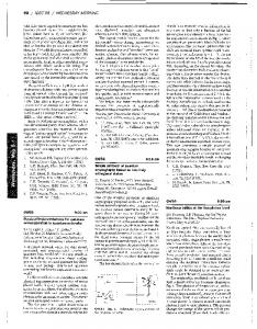
Modern classical computers would not be possible without Silicon semiconductor technology. It is therefore highly desirable to find a scheme for implementing quantum computation in some form of Silicon as integration of classical and quantum processing is a vital component of a large scale reliable quantum computer. Most Silicon-based schemes are two-dimensional by design and are believed to highly scalable (although several issues have been identified, see [12]), and thus a good candidate for Surface Codes. We will consider an architecture based on Silicon doped with ionized Phosphorus, for which a comprehensive description can be found in [12, 3]. The spin states of the donor electrons in a silicon substrate are used as qubits, yielding a relatively large coherence time of ' 60ms (which we will take as order ∼ 100ms). Efficient gate times on the order of ∼ 100ns are achieved through Coherent Transport by Adiabatic Passage (CTAP) schemes, yielding an 100ns approximate memory error rate of pmem ' 100ms = 10−6 . Finally, measurement time is estimated to be on the order of µs, and will use m = 100 gate times as a worst case scenario. Using these parameters, the times to failure were simulated as a function of pgate , as shown in figure 15. The error threshold was calculated to be 0.00968 ± 0.00021. It is interesting to observe the both Ion Traps and Silicon based architectures have yielded nearly identical threshold values for pthresh gate ! This is because, as consistent with our earlier discussion, the parameters used in both cases lies in the pgate  pmem , so both cases give a threshold pgate = 0 limit. Furthermore, in both cases memory time was not large value very close to the pmem enough to have a dominant effect on the threshold (as we saw earlier). For large scale architectures, the parameters used are likely to significantly worsen (at least at first!), and thresholds can thus be re-estimated from the general data collected. 4.3.3

Electrons on Helium

An advantage of the electrons on Helium implementation is the extremely large coherence times speculated. We therefore take T2 to be effectively infinite, and thus set our memory error to zero 26

Figure 16: Log-Log plot of Time to Failure versus Gate Error Rate for SiP (this will give a bound on the threshold for a real system with very small but finite memory error). Gates however are dipole based and relatively slow, taking 10ms. Hence, we also assume that tgate >> tmeas , and set measurement time m = 0. Both these approximations will serve to give an upper bound on the threshold for a real physical system with very small but finite memory error and measurement time. pgate Using these approximations, this case becomes equivalent to the pmem = 0( pmem → ∞) case thresh described earlier. The threshold for this case was found to be pgate = 0.0102 ± 0.0017. It is worth reemphasizing that this value is slightly higher than the uniform error threshold rate because memory errors have been turned off. With the introduction of non-zero measurement time and memory error rate, we expect this threshold to decrease, effectively moving along the surface shown in figure 14. We can therefore use the information obtained from our general threshold calculations to obtain a better estimate on the actual threshold value as more precise data becomes available.

4.4

Conclusion

We were successful in estimating the error rate threshold values for three distinct potential physical implementations of the surface code. In each case, error thresholds on the order of 1% were successfully demonstrated. Moreover, in each case we have effectively employed worst-case parameters, so the error rate threshold for an actual built system may even be better than expected. Each architecture was shown to possess very reasonable error rate thresholds. However, performing actual quantum computation with these architectures is another matter altogether. Scalability, transport times and fidelity, actual measurement fidelity all determine whether the surface code is most effectively implemented on a particular architecture. This is the subject of further research. We have confirmed the surface code to exhibit error thresholds several order of magnitude better than the previous best estimate on a two-dimensional lattice using the Stean code. Morover, we verified this for both the idealized case, and several physical implementations. The methodology employed is obtaining these results can easily be extended to any physical architecture suitable for the surface code. Moreover, the generalized results presented in this report allows for constant refinement of expected error rate thresholds as physical data of increased precision becomes available.

27

5

References

[1] A.M. Steane. How to Build a 300 Bit, 1 Giga-Op. Quantum Computer. quant-ph/0412165v2, 2006. [2] Peter Groszowski Austin Fowler, Ashley Stephens. High Threshold Universal Quantum Computation on the Surface Code. 12 March 2008. [3] B.E. Kane. A silicon-based nuclear spin quantum computer. 1998. [4] Goong Chen, David A Church, Berthold-Georg Englert, Carsten Henkel, Bernd Rohwedder, Marlan O Scully, and M Suhail Zubairy. Quantum computing devices: principles, designs, and analysis. CRC press, 2006. [5] D. Stick et. al. Ion Trap in a Semiconductor Chip. Nature Phys., (2):36–39, 2006. [6] Daniel Gottesman. Stabilizer Codes and Quantum Error Correction. PhD thesis, California Institute of Technology, 21 May 1997. [7] David Wang. private communication. [8] A. M. Steane et. al. D.M. Lucas. A long-lived memory qubit on a low-decoherence quantum bus. arXiv:0710.4421v1 [quant-ph], 21 October 2008. [9] E. Knill. Quantum Computing With Realistically Noisy Devices. Nature, 2005. [10] Andrew Landahl Eric Dennis, Alexei Kitaev. Topological Quantum Memory. Journal of Mathematical Physics, 43(9), 25 October 2002. [11] H. Haffner and W. Hansel et. al. Scalable multi-particle entanglement of trapped ions. Nature, 438:643, 2005. [12] Fowler AG Hollenberg LCL, Greentree AD. Two-dimensional architectures for donor-based quantum computing. PHYSICAL REVIEW B, 74(4), July 2006. [13] Dietrich Leibfried, Emanuel Knill, Signe Seidelin, Joe Britton, R Brad Blakestad, John Chiaverini, David B Hume, Wayne M Itano, John D Jost, Christopher Langer, et al. Creation of a six-atom schr¨ odinger catstate. Nature, 438(7068):639–642, 2005. [14] M. Nielsen and Isaaac Chuang. Quantum Computation and Quantum Information. Cambridge University Press, 2000. [15] M. Mosca P. Kaye, R. Laflamme. An Introduction to Quantum Computing. Oxford University Press, 2007. [16] P.L. Knight et. al. Ion Trap Quantum Gates, Decoherence and Error Correction. 7 September 2008. [17] J. Harrington R. Raussendorf. Topological Fault-Tolerance in Cluster State Quantum Computation. New J. Phys, 9(199), 1 February 2007. quant-ph/0703143. [18] K. Goyal R. Raussendorf, J. Harrington. A Fault-Tolerant One-Way Quantum Computer. Ann. Phys., 321:2242, 2006. [19] R. Raussendorf and J. Harrington. Fault-Tolerant Quantum Computation with High Threshold in Two Dimensions. Phy. Rev. Lett., 98, 14 May 2007. [20] D. james R. Stock. A scalable, high-speed measurement-based quantum computer using trapped ions. quant-ph/0605190v2 submitted to phy. rev. lett., 12 August 2008.

28

[21] Sergey Bravyi and Alexei Kitaev. Quantum Codes on a Lattice with Boundary. 1 February 2008. [22] W. Cook and A. Rohe. Computing Minimum-Weight Perfect Matching. INFORMS J. Computing, 11(138), 25 August 1999.

A

Partial C code

The simulator C code was implemented over ∼ 20 files. For brevity, only the main.c file is provided here. Further code can be provided on request of the author.

29

/* main.c * $Id: main.c 128 2008-10-01 00:56:35Z stuartah $ main.c 128 2008-06-21 00:56:35Z dswang $ * * Find the time to failure using blossom4 to find matching in surface * code error correction routine. */ #include #include #include #include #include #include #include #include



#include #include #include #include #include #include #include #include #include #include

"checkpoint.h" "component.h" "detect_fail.h" "error_corrector.h" "error_detector.h" "keep.h" "lattice.h" "simulator.h" "timer.h" "util.h"

typedef void (*make_lattice_func)(QUANTUM_COMPUTER *qc, int lx, int ly, bool **lattice); /*--------------------------------------------------------------*/ static void print_errors(QUANTUM_COMPUTER *qc, int lx, int ly, defect_t *d, FILE *stream) { int i, x, y; for (y = 0; y < ly; y++) { for (x = 0; x < lx; x++) { i = lx*y + x; if ((d->l < x && x < d->r) && (d->u < y && y < d->d)) { fprintf(stream, ". "); } else { fprintf(stream, "%c ", qc->qubit[i].x ? (qc->qubit[i].z ? 'y' : 'x') : (qc->qubit[i].z ? 'z' : 'I')); } } fprintf(stream, "\n"); } }

/*--------------------------------------------------------------*/ static void make_lattice_x(QUANTUM_COMPUTER *qc, int lx, int ly, bool **lattice) { int x, y; for (y = 1; y < ly; y += 2) { for (x = 1; x < lx; x += 2) lattice[y][x] = (qc->qubit[lx*y + x].x) ? true : false; } } static void make_lattice_z(QUANTUM_COMPUTER *qc, int lx, int ly, bool **lattice) { int x, y; for (y = 0; y < ly; y += 2) { for (x = 0; x < lx; x += 2) lattice[y][x] = (qc->qubit[lx*y + x].z) ? true : false; } } /*--------------------------------------------------------------*/ static void QC_Idle(QUANTUM_COMPUTER *qc) { int i; for (i = 0; i < qc->size; i++) QC_Timestep(qc, i); } static void duplicate_quantum_computer(QUANTUM_COMPUTER *src, QUANTUM_COMPUTER *dest) { int i; for (i = 0; i < src->size; i++) dest->qubit[i] = src->qubit[i]; } static void magic_intermediate(QUANTUM_COMPUTER *qc, int lx, int ly, int lt, defect_t *d, keep_t *keep, make_lattice_func make_lattice) { #define SWAP(a,b) do { bool **swap = a; a = b; b = swap; } while (0) make_lattice(qc, lx, ly, keep->lattice); find_match_intermediate(lx, ly, lt, d, keep); SWAP(keep->lattice, keep->lattice_ref); #undef SWAP }

static bool magic_final(QUANTUM_COMPUTER *qc, int lx, int ly, int lt, defect_t *d, keep_t *orig, keep_t *keep, make_lattice_func make_lattice, correction_func corrector, detection_func detector) { bool logical_op; duplicate_keep(lx, ly, orig, keep); make_lattice(qc, lx, ly, keep->lattice); find_match_final(lx, ly, lt, d, keep); apply_corrections(qc, keep->correction, corrector); logical_op = detector(qc, lx, ly, d); free_keep(ly, keep); return logical_op; } static void simulate_instance(QUANTUM_COMPUTER *qc, QUANTUM_COMPUTER *dup, int lx, int ly, defect_t *d, keep_t *keep_x, keep_t *keep_z, int *x_fail_time, int *z_fail_time) { bool x_fail = false; bool z_fail = false; int t; keep_t work; clear_keep(lx, ly, keep_x); clear_keep(lx, ly, keep_z); t = 1; while (!x_fail || !z_fail) { QC_Idle(qc); /* Pretend we are on the last step. Do special error free * syndrome detection. */ { duplicate_quantum_computer(qc, dup); /* Idle time step to simulate measurement error. */ dup->error_rate = qc->error_rate; QC_Idle(dup); dup->error_rate = 0.0; error_detect(dup, lx, ly, d); /* Check for X/Z failures. */ if (!x_fail) { if (magic_final(dup, lx, ly, t, d, keep_x, &work, make_lattice_x, QC_X, smooth_detect_logicalx)) { x_fail = true; *x_fail_time = t;

} } if (!z_fail) { if (magic_final(dup, lx, ly, t, d, keep_z, &work, make_lattice_z, QC_Z, smooth_detect_logicalz)) { z_fail = true; *z_fail_time = t; } } } /* If we are still alive, then we do regular error detection * using the ancillas. Do not error correct or check for * logical failure. */ { /* Idle time step to simulate measurement error. */ error_detect(qc, lx, ly, d); QC_Idle(qc); /* Check for X/Z failures. */ if (!x_fail) { magic_intermediate(qc, lx, ly, t, d, keep_x, make_lattice_x); } if (!z_fail) { magic_intermediate(qc, lx, ly, t, d, keep_z, make_lattice_z); } } t++; } } static void simulate_instances(int lx, int ly, defect_t *d, double error_rate, int instance, int total_instances) { QUANTUM_COMPUTER qc; QUANTUM_COMPUTER dup; keep_t keep_x; keep_t keep_z; int x_fail_time = INT_MAX; int z_fail_time = INT_MAX; components_init(); make_keep(lx, ly, &keep_x); make_keep(lx, ly, &keep_z); for (; instance < total_instances; instance++) { checkpoint(instance);

QC_Startup(&qc, lx*ly, error_rate); QC_Startup(&dup, lx*ly, error_rate); simulate_instance(&qc, &dup, lx, ly, d, &keep_x, &keep_z, &x_fail_time, &z_fail_time); fprintf(stdout, "(%d, %d)\n", x_fail_time, z_fail_time); fflush(stdout); QC_Shutdown(&dup); QC_Shutdown(&qc); } free_keep(ly, &keep_x); free_keep(ly, &keep_z); components_shutdown(); } /*--------------------------------------------------------------*/ static void usage(char *progname) { fprintf(stderr, "usage: %s [-h] [options]\n\n" "Options:\n" " -d \tset the code-word distance\n" " -n \tset the number of instances to run\n" " -p \tset the error probability\n" " -s \tset the random number seed\n" " -S \trestore the state of a terminated computation\n", progname); } static void prefab(int dist, int *lx, int *ly, defect_t *d) { int du, dd, dl, dr; int xdist, zdist; if (dist