Apr 18, 2002 ... The most basic definition of a wavelet is simply a function with a well defined
temporal ... This is a rich library of Matlab functions dealing with.
EE482C: Advanced Computer Organization Stream Processor Architecture Stanford University Homework #1: Due Date: Checkpoints:
Homework #1 Thursday, 18 April 2002
Wavelet Compression on Imagine Tuesday, 30 April 2002 Tuesday, 23 April 2002; Friday, 26 April 2002
The purpose of this assignment is to give you a feel for stream programming. To achieve this, you will program a simple application for Imagine using the Imagine tool chain. The application is a one-dimensional signal compression based on wavelets. Please work on this assignment in groups of up to four people, and hand in one write-up per group. I’ll give a very brief introduction to wavelets and wavelet compression, and then a more detailed description of the algorithm you will implement. If you are interested in what exactly is required in this assignment, go to Section 3 on page 6.
1
What is Wavelet Compression
This section provides a very brief description of compression using wavelets.
1.1
What are Wavelets
The most basic definition of a wavelet is simply a function with a well defined temporal support that “wiggles” about the x−axis (it has exactly the same area above and below the axis). This definition however does not help us much, and a better approach is to explain what the wavelet transform and wavelet analysis are. The basic Wavelet Transform is similar to the well known Fourier Transform. Like the Fourier Transform, the coefficients are calculated by an inner-product of the input signal with a set of orthonormal basis functions that span �1 (this is a small subset of all available wavelet transforms though). The difference comes in the way these functions are constructed, and more importantly in the types of analyses they allow. The key difference is that the Wavelet Transform is a multi-resolution transform, that is, it allows a form of time–frequency analysis (or translation–scale in wavelet speak). When using the Fourier Transform the result is a very precise analysis of the frequencies contained in the signal, but no information on when those frequencies occurred. In the wavelet transform we get information about when certain features occurred, and about the scale characteristics of the signal. Scale is analogous to frequency, and is a measure of the amount of detail in the signal. Small scale generally means coarse details, and large scale means fine details (scale is a number related to the number of coefficients and is therefore counter-intuitive to the level of detail). The Discrete Wavelet Transform can be described as a series of filtering and subsampling (decimating in time) as depicted in Figure 1. In each level in this series, a set
2
EE482C: Homework #1
Figure 1: Discrete Wavelet Transform (from http://www.public.iastate.edu/
∼rpolikar/WAVELETS/WTpart4.html
of 2j−1 coefficients are calculated, where j < J is the scale and N = 2J is the number of samples in the input signal. The coefficients are calculated by applying a high-pass wavelet filter to the signal and down-sampling the result by a factor of 2. At the same level, a low-pass scale filtering is also performed (followed by down-sampling) to produce the signal for the next level. Both the wavelet and scale filters can be obtained from a single Quadrature Mirror Filter (QMF) function that defines the wavelet. Each set of scale-coefficient corresponds to a “smoothing” of the signal and the removal of details, whereas the wavelet-coefficients correspond to the “differences” between the scales. Wavelet theory shows that from the coarsest scale-coefficients and the series of the wavelet-coefficients the original signal can be reconstructed. The total number of coefficients (scale + wavelet) equals the number of samples in the signal.
EE482C: Homework #1
1.2
3
Wavelet Compression
How do we use these transform coefficients to perform compression? The distribution of values for the wavelet coefficients is usually centered around 0, with very few large coefficients. This means that almost all the information is concentrated in a small fraction of the coefficients and can be efficiently compressed. This is done by quantizing the values based on the histogram and encoding the result in an efficient way, e.g. Huffman Encoding. For this homework we will use a simpler method, and instead of quantizing we will discard all but the M largest coefficients. This provides a compression ratio of roughly 2M/N (the factor of 2 is for storing both the coefficient value and index).
1.3
Where to Get More Information
A very good book on wavelets is “A Wavelet Tour of Signal Processing, 2nd edition” by St´ ephane Mallat. I also found several reasonable tutorials on the web such as: • cas.ensmp.fr/∼chaplais/Wavetour presentation/Wavetour presentation US.html • http://www.public.iastate.edu/∼rpolikar/WAVELETS/WTtutorial.html • http://perso.wanadoo.fr/polyvalens/clemens/wavelets/wavelets.html
2
Algorithm Description
The compression algorithm has two parts. The first is a wavelet transform that uses the Fast Wavelet Transform taken from the Wavelab library developed at the Statistics Department here at Stanford. This is a rich library of Matlab functions dealing with wavelets and wavelet analysis, and you are encouraged to check out their web page at http://www-stat.stanford.edu/ wavelab/. After calculating the transform coefficients a sort is applied, and all but the largest n coefficients are discarded. The signal can be reconstructed by performing an Inverse Wavelet Transform using the n stored coefficients and zeroing out all other coefficients. I will now describe in more detail the simplest wavelet transform which is an orthogonal and periodic transform, and implemented by the FWT PO.m function. You can find this function and the entire Wavelab distribution in /afs/ir.stanford.edu/class/ee482c/wavelab/Orthogonal. The pseudocode for the Fast Wavelet Transform algorithm appears below. The algorithm consists of a main loop that has two parts. This first part calculates the wavelet coefficients in the current scale (high-pass filter), and the second part calculates the scale coefficients by low-pass filtering and essentially shifts the scale down (towards less details). This loop is repeated O(log n) times, once for each scale. Notice that the amount of computation in each iterations shrinks by a factor of two for each scale lowered. As a result the total computation cost is O(n), and the filter is applied to roughly 4n elements.
EE482C: Homework #1
4
Both the low-pass and high-pass filtering are performed on a periodically padded version of the current-scale signal (ϕj (n)), and the result is decimated by 2. The filter kernels define the wavelet and are computed from its characteristic QMF.
2.1 // // // // // // // // // // //
Fast Wavelet Transform Pseudocode
I’ve used some Matlab like notation: 1. Arrays are indexed from 1 to their length instead of 0 - (length - 1) 2. x(start:end) means all elements of x from start index to end index 3. [x y] mean concatenate y to x 4. x + 1 means add 1 to all elements of x 5. [start:end] is a vector which includes all numbers from start to end 6. x(y) - a vector of elements of x with indices y 7. [start:stride:end] a vector from start to end with a constant stride [1:2:10] = [1 3 5 7 9]
function WFT(x, qmf) { // x - input signal // qmf - qmf of the wavelt function for (i = 1; i