We know from Information theory that good predictors form good Compressors [2]. We know that Recurrent Neural Networks (
DeepZip: Lossless Compression using Recurrent Networks Kedar Tatwawadi Stanford University
[email protected]
Abstract There has been a tremendous surge in the amount of data generated. New types of data, such as Genomic data [1], 3D-360 degree VR Data, Autonomous Driving Point Cloud data are being generated. A lot of human effort is spent in analyzing the statistics of these new data formats for designing good compressors. We know from Information theory that good predictors form good Compressors [2]. We know that Recurrent Neural Networks (LSTM/GRU) based models are good at capturing long term dependencies [3], and can predict the next character/word very well. Thus can RNNs be efficiently used for compression? We analyze the usage of Recurrent Neural Networks for the problem of Data Compression. DeepZip Compressor consists of two major blocks: RNN based probability estimator and Arithmetic Coding block [4]. In the first section, we discuss existing literature and the basic model framework. We then take a look at experiment results on synthetic as well as real Text and Genomic datasets. Finally, we conclude by discussing the observations and further work. Code: https://github.com/kedartatwawadi/NN_compression
1
Introduction
The Big Data revolution has led to collection of huge amounts of different types of datasets such as images, texts etc. New types of data formats, such as 3D VR data, point cloud data for autonomous driving mapping, various types of genomic data [1] etc. are also being generated in huge proportions. Thus, there is a need for coming up with statistical models and efficient compressors for these data formats. There have been significant advancement on the problem of lossless compression in the past 50 years. In his seminal work [5], Claude Shannon showed that the Entropy rate is the best possible compression ratio for the given source, and gave a methodology to achieve it (although impractical). J. Rissanen proposed Arithmetic coding [4], which is an efficient procedure for achieving the Entropy bound for known distributions. For sources with unknown distributions (like text, DNA sources), adaptive variants [6] of Arithmetic encoding have also been designed, which try to compress by learning the conditional k−gram model distribution. However, as the complexity increases exponentially in k, generally the context is limited to k = 20 symbols. This can lead to a significant loss of compression ratio, as the models are not able to capture long term dependencies. We know that Recurrent Neural Network (LSTM/GRU) based models are good at capturing long term dependencies [3], and can predict the next character/word very well. Thus, can RNN based frameworks be used for compression? In this work, we explore and understand the utility of RNN based language models along with Arithmetic coding to improve lossless compression 1
1.1
Past Work
There has been some related work in the past on the lossless compression using Neural networks. Schmidhuber et.al.[7] discussed the application of character-level RNN model for text, and observed that it gives competitive compression performance as compared with the existing compressors. However, as Vanilla RNN’s were used, the performance was not very competitive for complex sources with deeper dependencies. Also, the models required significant amount of training time (close to 50 epochs) which made them slightly impractical. Mahoney et.al [8] came up with a different framework for using neural networks for Text compression. An RNN was used as a context mixers for mixing the opinions of multiple compressors, quite a few of which are specific to text data. Similar approach was improved by the CMIX[9] compressor, which mixes together more than 2000 models using an LSTM context mixer. This approach can be seen as a kind of Boosting over multiple compressor experts, and thus leads to improved performance. However, it still requires designing of the individual context based compressors, which can depend a lot on the kind of source being analyzed. Recently there has also been some work on application of more complex models (word-based and semantically aware models) for text compression [10].
Figure 1: LSTM’s used as context mixers in the CMIX Compressor for mixing together several compression models In this work, we first analyze and understand the performance of RNN & Arithmetic Coding based compressors on synthetic datasets, with known entropy. The aim of the experiment was to gain good intuitive understanding of the capabilities and limits of various RNN structures. We also perform experiments on pseudo random number generated sequences (PRNG)[11], which although have 0 entropy rate (since they are deterministic), however are very difficult to compress using standard techniques. Based on the understanding derived from the previous experiments on synthetic datasets, we employ the models for compression of Text, and genomic datasets.
2 2.1
Compressor Framework Overview
We first take a look at the compressor model we used for the experiments. The framework can be broken down into two blocks: 1. RNN Probability Estimator block: For a data stream S0 , S1 , . . . , SN , the RNN probability estimator block estimates the conditional probability distribution of Sk , based on the previously observed symbols S0 , S1 , . . . , Sk−1 . This probability estimate Pˆ (Sk |S0 , S1 , . . . , Sk−1 ) is fed into the the Arithmetic encoding block. 2
2. Arithmetic Coder Block: The Arithmetic coder block can be thought of as an FSM which takes in the probability distribution estimate for the next symbol and encodes it into a state (decoder operations are reversed)
2.2
RNN Probability Estimator Block
In practice, the RNN Estimator block can be any Recurrent Neural Network block (LSTM/GRU) which has a Softmax layer at the end for probability estimation. The Arithmetic Coder block can be the Vanilla Arithmetic Coding FSM, or can be replaced by a faster Asymmetric Numeral Systems (ANS) block [12]. There are a couple of important constraints with respect to operations of the model: 1. Causality of Input: The RNN Estimator needs to be causal, and can have input as features based only on only on the previously encoded symbols (BiLSTM etc. might not work). 2. Weights Update: The Weights update (if performed) should be performed exactly in the encoder and the decoder. This is required, as we need both the encoder and decoder to produce the same distributions for every symbol. We majorly explore two models, the Character level GRU model (DeepZip-ChGRU) and the Features based model (DeepZip-Feat). In the DeepZip-GRU, at the k th step, the input to the GRU blocks is Xk−1 and the statek−1 which is the state output of the model until that point. The DeepZip-Feat consists of inputs as features computed causally, such as past 20 symbols, and context appearance counts in the observed stream. Other models which we briefly consider are word-based models, Attention-RWA[13] models.
2.3
Arithmetic Coder Block
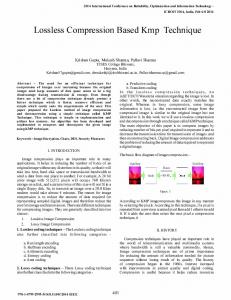
The Arithmetic encoder maintains a range in the interval [0, 1]. Every stream of symbols uniquely determine a range. This range can be computed sequentially and is directly based on the probability estimate for the next symbol. This range can be considered as a state of the Arithmetic Encoder, which is transmitted to the next iteration. At the end, this range is encoded which forms the compressed data. The decoding operations are inverse operations, given the probability estimates. The Arithmetic encoding operations are illustrated in Fig[2] (More details can be found in the cited references).
Figure 2: Arithmetic Encoding of the sequence (0, 2, 3) for an i.i.d (0.6, 0.2, 0.1, 0.1) distributed source [source: Wikipedia] 3
¯ AE (average number of bits used per symbol) of the Arithmetic encoder Also, the compression size L is very close to the normalized cross-entropy loss of the RNN based estimator (see Eq[1]). Thus, CE-loss is infact the optimal loss function for this framework. ¯ AE ≤ 1 log2 1 + 2 L N pˆ(S N ) 2.4
(1)
Encoder & Decoder Operations
The Encoder and decoder operations are illustrated in the figures below: 1. The Arithmetic Encoder block always starts with a Default probability distribution estimate for the first symbol S0 . This is done so that the Decoder can decode the first symbol. 2. Both the Arithmetic Encoder and the RNN Estimator blocks pass on the state information across iterations. The final state of the Arithmetic Encoder acts as the compressed data. 3. If the model is trained for more than an epoch, the weights of the RNN Estimator Block also need to be stored, and would count in the compression size (MDL Principle [14])
Figure 3: Encoder Model Framework
3
Experiments on Synthetic Datasets
We experiment with synthetic sources with known Entropy. As Entropy acts as a lower bound on the compression ratio, thus working with synthetic sources enables us to gauge the performance of different models against this ideal bound. 1. i.i.d Sources: We consider i.i.d sources of variety of distributions. As existing compressors do well on this, the minimum expectation is RNN’s will do well. 2. Markov-k sources: Markov-k sources are 0-entropy sources with markovity of k. They are governed by Xn = Xn−1 + Xn−k
mod M
(2)
Markov-k sources are difficult to compress, as until order k, they have empirical entropy close to 1 (almost uniform samples). 4
Figure 4: Decoder Model Framework We next discuss some interesting experiments with a variety of models on the above datasets. The models which we explore are as follows: 1. DeepZip-ChRNN: The Character-level-RNN based neural network model. 2. DeepZip-ChGRU: The Character-level GRU based neural network model 3. DeepZip-Feat: The GRU based model, which takes in features which are function of all previously observed symbols instead of just the previous input. For example, we consider Features such as last 50 symbols, and 4 symbol context counts for 5 different contexts. 3.1
IID Sources
IID data sources seemed very simple for even the smallest Vanilla-RNN based networks to optimize. This is expected, considering the model itself does not need any kind of memory. The DeepZipChGRU model with size 16-cells reaches the entropy bound in a few iterations. 3.2
Vanilla-RNN based models
We consider a Vanilla-RNN based 128-cell DeepZip-ChRNN model on Markov-k sources. The implementation details are as follows: 1. Only random seed is Stored: The model is initialized using a stored random seed, which is also communicated to the decoder. Thus, the effectively the model weights do not contribute to the total compressed data size. 2. State preservation: We train the model weights during the encoding as well as decoding using truncated backpropagation of sequence length 50. The state of the RNN is preserved across batches, and is used appropriately for the next sequential batch 3. Weights training is replicated: Both the encoder and the decoder perform training of the weights in the exact same fashion to replicate the probability estimates and thus achieve lossless compression (Adam Optimizer with the same learning rate is used) 4. Single Pass: As we do not store the weights of the model, we perform a single pass (1 epoch) through the data Fig[5] shows the performance of the DeepZip-ChRNN model. We see that DeepZip-ChRNN performs extremely well on Markov-k datasets until markovity k = 30. In fact DeepZip-ChRNN model 5
Figure 5: Performance of DeepZip-ChRNN-128-Cell model on Markov-k sources performed better (faster convergence to entropy) than DeepZip-ChGRU models which is slightly surprising. However, the model is not able to learn at all dependencies more than 30 timesteps away, and thus performs no compression for Markov-35 source. This in a sense showcases the vanishing gradients issue in the Vanilla-RNN models. 3.3
LSTM/GRU based Character-level models
We experiment with LSTM/GRU based probability Estimator models. The DeepZip-ChGRU 128cell model has similar implementation details (and training procedure) as for Vanilla RNN described in section[3.2].
Figure 6: Performance of DeepZip-ChGRU-128-Cell model on Markov-k sources Fig[6] shows the performance of the DeepZip-ChGRU on Markov-k sources. DeepZip-ChGRU is able to compress Markov-50 sources, which is better than the performance of DeepZip-ChRNN. Essentially it is able to capture dependence upto 50 timesteps. This raises a question if this was again due to the vanishing gradients issue in GRU, or due to the training procedure where we truncate the backpropagation to 50 timesteps (as mentioned in Section [3.2]). To understand the impact of the sequence length of the truncated backpropagation, we train the same DeepZip-ChGRU network with sequence length of 8. In that scenario, the network was able to compress only Markov-20 sources, and not better! Thus, we concluded that although the network can learn dependencies longer than the sequence length, it still gets very difficult after 6
Comparison of DeepZip performance with Other Compressors Dataset Markov-20 Markov-30 Markov-50 Markov-80 Markov-100 Markov-140
Size
DeepZip-ChGRU
DeepZip-Feat
GZIP
Adaptive-AE
100MB 100MB 100MB 100MB 100MB 100MB
200KB 1MB 30MB 100MB 100MB 100MB
200KB 400KB 500KB 2MB 38MB 100MB
5MB 40MB 63MB 69MB 100MB 100MB
2MB 87MB 100MB 100MB 100MB 100MB
Figure 7: Performance of DeepZip-128-Cell models are compared with GZIP[15] and Adaptive Arithmetic Coding-CABAC approximately 2 times the sequence length. We also tried sequence length of 100, which helps a bit, as DeepZip-ChGRU is able now to compress Markov-60 sources, but it does not improve performance on Markov-70 sources. Thus, this experiment suggests that GRU’s face vanishing gradients at around 70 timesteps. 3.4
Feature based models
In the previous section, we saw that GRU’s face vanishing gradients problem, and thus do not compress Markov-60 sources. This is also summarized in Fig[7], which shows the performance of DeepZip-ChGRU on Markov-k sources, and also compares it with standard compressors such as GZIP[15], and 24bit-CABAC[16] or Context-Adaptive-Binary-Arithmetic-Compressor. We observe that GZIP is able to compress Markov-80 sources to some extent. This motivates the use of context counts as features, to circumvent the issue of vanishing gradients. We thus consider the DeepZip-Feat model which has as inputs past 50 symbols (instead of only 1), and 5 4-gram context counts. Fig[7] results show that the DeepZip-Feat model does face vanishing gradients issue, but for more difficult sources like Markov-140. We observe that in most of the cases, the DeepZip models outperform GZIP and Adaptive arithmetic encoder models for the Markov-k sources.
4
Experiments on Practical Datasets
Based on the insights gained from experimenting with Markov-k synthetic sources, we next experiment on some practical datasets which includes: 1. PSRN-m-n: We experiment with the Lagged Fibonacci Pseudo-Random-NumberGenerated sequences (PSRN)[19]. As they are practically ”random numbers”, it is a difficult dataset to compress! 2. Hutter Prize dataset: The 50,000 EUR prize competition wikipedia text dataset [17] 3. Enwiki9: A larger XML Wikipedia Dump [18] 4. HGP-Chr1: The Human Genome Project DNA Chromosome-1 reference [19]. The Chromosome-1 is a difficult source as it is well known that genome sequences although have significant repeats, they are significantly separated (few 100s to 10,000 symbols). There are also structured artifacts such as palindromes etc. The results are summarized in Fig[8]. For the Pseudo-random-number-generated sequences (PRNG) experiment, we choose the parameters with the highest repeat length [11] (i.e. more difficult). We observe that the GZIP performs poorly on the PRNG sequences, which is not completely unexpected considering they are almost ”random”. Also notice that DeepZip-Feat models are able to compress the PRNG-73-31 sequences significantly, and hence are able to figure out that PRNG-73-31 is not actually ”random” which is a pretty interesting thing. We also observe that DeepZip-Feat is able to perform better than the existing best custom DNA sequence compressor MFCompress [20] (although the compression/decompression times are sig7
Comparison of DeepZip performance on PRNG & Real datasets Dataset PRNG-31-13 PRNG-52-21 PRNG-73-31 Hutter-Prize EnWiki-9 Chromosome-1
Size
DeepZip-ChGRU
DeepZip-Feat
GZIP
Best-Custom
100MB 100MB 100MB 100MB 1GB 240MB
32MB 85MB 100MB 18MB* 178MB 48MB
500KB 1MB 62MB 16.5MB* 168MB 42MB
95MB 100MB 100MB 34MB 330MB 57MB
– – – 15.9MB (CMIX) 154MB (CMIX) 49MB (MFCompress)
Figure 8: Performance of DeepZip-128-Cell models on practical datasets
nificantly slower for DeepZip). DeepZip is not able to perform better on the Text datasets, possibly because text data does not have very long dependencies (rarely has dependencies beyond 100 characters 2 sentences).
5
Conclusion & Further Work
We performed experiments mainly using two different models, a character-level GRU model and a feature based GRU model. Both of the models performed significantly well on difficult sources such as pseudo-random-number sequences (PRNG). The results highlight potential for lossless compression using RNN based models. The challenge is to make the models faster and work well on more complex sources. One interesting extension of the project would be working with lossless compression of images. Images have significant dependencies, and modeling the same with RNN should be beneficial, as demonstrated in [21]. A fun extension would be breaking (no-more-random)more complex Pseudorandom-number generators! Acknowledgments I would like to thank my mentor Arun Chaganty for helpful discussions. I would also like to thank Microsoft for providing GPUs. References [1] Nature Article on Genomic Boom: http://www.nature.com/news/ genome-researchers-raise-alarm-over-big-data-1.17912 [2] EE376C Lecture Notes: Universal Schemes in Information Theory: http://web.stanford.edu/ class/ee376c/lecturenotes/intro_lecture_slides_ee376c_fall_2016_2017.pdf [3] Unreasonable Effectiveness rnn-effectiveness/
of
RNN:
http://karpathy.github.io/2015/05/21/
[4] Rissanen, Jorma, and Glen G. Langdon. ”Arithmetic coding.” IBM Journal of research and development 23.2 (1979): 149-162. [5]Shannon, Claude Elwood. ”A mathematical theory of communication.” ACM SIGMOBILE Mobile Computing and Communications Review 5.1 (2001): 3-55. [6] Witten, Ian H., Radford M. Neal, and John G. Cleary. ”Arithmetic coding for data compression.” Communications of the ACM 30.6 (1987): 520-540. [7] Schmidhuber, Jrgen, and Stefan Heil. ”Sequential neural text compression.” IEEE Transactions on Neural Networks 7.1 (1996): 142-146. [8] Mahoney, Matthew V. ”Fast Text Compression with Neural Networks.” FLAIRS Conference. 2000. APA [9] CMIX : http://www.byronknoll.com/cmix.html
8
[10] Cox, David. ”Syntactically Informed Text Compression with Recurrent Neural Networks.” arXiv preprint arXiv:1608.02893 (2016). APA [11] Knuth, Donald Ervin. The art of computer programming: Vol. 2. Pearson Education. [12] ANS: Duda, Jarek. ”Asymmetric numeral systems.” arXiv preprint arXiv:0902.0271 (2009). [13] Ostmeyer, Jared, and Lindsay Cowell. ”Machine Learning on Sequential Data Using a Recurrent Weighted Average.” arXiv preprint arXiv:1703.01253 (2017). [14] Grunwald, Peter. ”A tutorial introduction to the minimum description length principle.” arXiv preprint math/0406077 (2004). APA [15] GZIP: Deutsch, L. Peter. ”GZIP file format specification version 4.3.” (1996). [16] CABAC: Prakasam, Ramkumar. ”Context adaptive binary arithmetic code decoding engine.” U.S. Patent No. 7,630,440. 8 Dec. 2009. [17] Hutter Prize: http://prize.hutter1.net/ [18] Enwiki9: http://www.mattmahoney.net/dc/textdata [19] HGP: Sawicki, Mark P., et al. ”Human genome project.” The American journal of surgery 165.2 (1993): 258-264. [20] MFCompress: Pinho, Armando J., and Diogo Pratas. ”MFCompress: a compression tool for FASTA and multi-FASTA data.” Bioinformatics 30.1 (2014): 117-118. [21] PixelRNN: Oord, Aaron van den, Nal Kalchbrenner, and Koray Kavukcuoglu. ”Pixel recurrent neural networks.” arXiv preprint arXiv:1601.06759 (2016).
9