RScaLAPACK: High-Performance Parallel Statistical Computing with R and ScaLAPACK Srikanth Yoginath1,2, David Bauer1,2, Nagiza Samatova1,3, Guruprasad Kora1, George Fann, and Al Geist1 Abstract
With the growing popularity of parallel computation, researchers are looking for various means to reduce the problem solving time by performing the computations in parallel. While, interested in parallel computation they do not want to deal with the parallel programming complexities. In this paper, through RScaLAPACK we demonstrate a means that enables the user to carryout parallel computation without dealing with the intricacies of parallel programming. The name RScaLAPACK is made up of two distinct words, R and ScaLAPACK. The first word stands for the software that provides an environment and a language for statistical computing and graphics. This Open source software has developed rapidly and has been extended by a large collection of packages. The second word ScaLAPACK stands for a library of high-performance linear algebra routines for distributed-memory message passing MIMD computers and networks of work stations supporting PVM and/or MPI. As the name suggests, RScaLAPACK is a library built for the R statistical environment using the ScaLAPACK library. Through RScaLAPACK the
user can setup the parallel environment, distribute data and carry out the required parallel computation using a single R function call. While the interface maintains the look and feel of the R system, RScaLAPACK allows carrying out analyses with a performance that scales well with both the problem size and the number of processors. RScaLAPACK is developed using C and FORTRAN languages and is distributed as an add-on library to the R statistical package. It is made available as an Open Source package and can be found at http://www.aspect-sdm.org/Parallel-R or on R’s CRAN web site http://www.r-project.org. In this paper we discuss the design, working and performance characteristics of the RScaLAPACK library. 1. Introduction
To address the ever increasing computational and memory requirements of scientific data analysis, a scalable parallel solution to the problem is highly desirable. Currently, most of the mathematical packages are moving toward parallel computation as a solution to meet the ever increasing computational demands of their users efficiently [1-2], The R [3] software that provides a language and an environment for statistical computing [3-4] is one such package. Apart from providing a wide variety of statistical and graphical techniques, it is highly extensible. However, at present, R has a limited support for parallel computation. Several R add-on packages like Rmpi [5] and rpvm [6] provide building blocks for writing parallel programs using the native programming language. These packages are in turn used to build parallel libraries like snow [7] that addresses the embarrassingly parallel statistical computations. Even though this approach of development makes parallel computation possible performance wise they could be less efficient as they use interpreted code for writing parallel libraries and their usage does not make the parallel computations transparent to the user. 1
Computer Science and Mathematics Division, Oak Ridge National Laboratory, Oak Ridge, TN 37830 Both authors have contributed equally to this work 3 Corresponding author:
[email protected]
2
1
Our work is driven by the need to provide a completely transparent parallel computational capability to the user. Toward this goal, one approach is to capitalize on the existing libraries that perform parallel computations efficiently and make them accessible within R through an easy-to-use interface. The ScaLAPACK [8-9] library that provides function APIs to the parallel high-performance linear algebra routines maps well to this task. Further its serial counterpart the LAPACK [10] that is being used as an underlying mathematical library by many statistical analysis routines in R serves as a roadmap for this work. On the other hand the usage of the ScaLAPACK library demands the user to perform a number of tasks like, process grid setup; input data decomposition and distribution among different processes; final result collection and aggregation; along with many other well-defined minor details that needs to be carried out before and after the actual ScaLAPACK function call. With the RScaLAPACK we reduce all the above tasks into a single instruction in the R environment. This way we also get rid of the burden of details that a general user is expected to know to use any of the ScaLAPACK library routines. In addition, the evaluated result using RScaLAPACK routines are in the form of R-objects and hence, can be used for further analysis using the diverse collection of analysis routines provided by R. In this paper we discuss the overall architecture, the function call support, and the performance of the RScaLAPACK package. Sections 2 and 3 discuss R and ScaLAPACK, respectively, highlighting the flexibility provided by the former and the complexity involved in the usage of the latter that influences the development of a system like RScaLAPACK. In Section 4 we discuss the architecture of the RScaLAPACK system. A description of the current functionalities and implementation details follows in Section 5. In section 6, we examine the performance gain and observed speedup of RScaLAPACK. We conclude with Section 7. 2. The R Statistical Package R is an Open Source interactive programming environment for data analysis and graphics. It is one of the most widely used statistical data analysis packages. It provides an effective data handling and storage facility; a suite of operators for calculations on arrays and matrices; a large, coherent, integrated collection of intermediate tools for data analysis; > > library(stats) # Load the stats package. graphical facilities for data > results # analysis on a matrix “USArrests” that is provided by dataset package. developed simple > summary( results ) # Print the summary of the prcomp result. programming language that > includes conditionals, Figure 1.a. Sequence of R commands to perform Principal loops, user defined recursive functions, as well Component Analysis on a given matrix. as input and output capabilities. R package > comprises of many > dyn.load( “foo.so”) # Load the shared library. classical and modern > .C( “foobar” ) # Execute the C function foobar. > : statistical techniques. Some > .Fortran( “foobar2” ) #Execute the FORTRAN function. of these are built into the > : base R environment but > dyn.unload( “foo.so” ) #Unload the shared library foo.so many are supplied as > optional add-on packages, Figure 1.b. A simple code that depicts loading, unloading, and usage of an external object code in R.
2
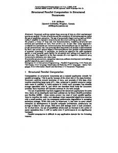
like the stats package that provides a rich suite of data analysis routines (Figure 1.a). It has a dialect of the S language created by AT&T Bell Laboratories [18] and is freely distributed under the terms of GNU General Public License. Of all the above mentioned capabilities of R, the interesting one to our concern is its extensibility characteristic. Through the concept of Packages R provides the mechanism for loading optional code and attached documentation as needed. Further, R provides a function interfaces to the compiled code that has been linked into R. The compiled code in the form of shared objects in UNIX (or DLLs in Windows) can be easily loaded and unloaded from the R environment using simple R function calls (Figure 1.b). This feature allows the developers to build a system in C, C++, or FORTRAN languages and provide the R interfaces to the compiled code, through which the system could be controlled, thus making the system details transparent to the user. Such systems can be distributed as R’s add-on packages. Once installed, they can be used optionally by loading them into the environment as required. We have taken advantage of this feature of R to develop RScaLAPACK package in providing a transparent parallel platform for R users as described in later sections. 3. The ScaLAPACK Library ScaLAPACK is designed to give high efficiency on MIMD distributed memory concurrent supercomputers. In addition, the software is designed so that it can be used with clusters of workstations through a networked environment and with a heterogeneous computing environment via PVM or MPI . The ScaLAPACK routines are based on block-partitioned algorithms in order to minimize the frequency of data movement between different processes, which helps reduce the fixed startup cost incurred each time a message is communicated. The fundamental building blocks of ScaLAPACK library are parallel versions of the Level1, Level2, and Level3 BLAS, called the Parallel BLAS, or PBLAS, and a set of Basic Linear Algebra Communication Subprograms (BLACS) for communication tasks that arise frequently in parallel linear algebra computations. ScaLAPACK can solve systems of linear equations, linear least square problems, eigenvalue problems, and singular value problems. It provides a set of FORTRAN APIs for carrying out the parallel computation. To carry out the computation, a two dimensional rectangular grid encompassing all the processes involved in the parallel computation is first created. The rectangular grid is often referred to as the process grid. This is followed by block-cyclic data distribution of the input matrix, which involves the decomposition of the matrix into small rectangular blocks starting at its upper left corner and their uniform distribution in each dimension of the process grid. Figure 2 shows an example of a twodimensional block cyclic distribution of the elements of a 16x16 matrix with a block size of 2x2 distributed over a process grid of dimension 2x2.. To start with the matrix of dimension 16x16 is divided into data-blocks each of dimension 2x2. This results an 8x8 matrix with each element as a data-block of size 2x2 as shown in Figure 2. Now, this matrix is distributed block by block, among the different processes of the two-dimensional process grid in a cyclic fashion. The resulting pattern of distribution of the data-blocks of the global matrix can be seen in the Figure 2, where each data-block of the global matrix holds the rank of the process to which it is assigned.
3
0 2 0 2 0 2 0 2
1 3 1 3 1 3 1 3
0 2 0 2 0 2 0 2
1 3 1 3 1 3 1 3
0 2 0 2 0 2 0 2
1 3 1 3 1 3 1 3
0 2 0 2 0 2 0 2
1 3 1 3 1 3 1 3
All ScaLAPACK routines assume that the data has been distributed on the process grid prior to the invocation of the routine. After a ScaLAPACK routine completes the computation, the results still distributed across the process grid need to be collected.
In summary, the user is expected to do the task of process grid creation, data distribution, result collection and the process grid release for using the high performance ScaLAPACK routines. The RScaLAPACK system takes Figure 2. Two-dimensional block-cyclic distribution of a 16x16 matrix using 2x2 care of all the additional tasks involved in using the ScaLAPACK routines and provides easy access to these process grid and block size of 2x2. high performance routines through a single R function call, thus making the parallelism transparent to the user. 4. The RScaLAPACK Architecture The requirement of performing computations outside parent R process to support the ability to perform computations on large data sets and the need for an entity to manage the execution of these external processes led to the current architecture. The computational entity running outside the parent R process is referred to as Spawned Process(es) (Figure 3) and it could be any parallel computational system with a well-defined data distribution and result collection strategies . The management entity, which we call as Parallel Agent (PA) (Figure 3), orchestrates the data flow between R environment and the parallel computational unit. The Parallel Agent was developed under the design consideration that it should provide a single window entry-point to the R environment for data handling while it provides a platform to plug-in a generic parallel computational system. The current implementation uses the ScaLAPACK as it computational unit, thus the name RScaLAPACK.
Figure 3. RScaLAPACK architecture. All requests for RScaLAPACK functions are forwarded to the Parallel Agent (PA). Upon the request from the user, the PA spawns the requested number of processes,
distributes the input data across the process grid (as per input instructions), collects the result from the process grid, and returns it back to the user as an R object. The Spawned Processes are the worker processes that work in coordination with each other and the PA. As per the instructions from the PA, the Spawned Processes create the process grid, receive the distributed data-blocks from the PA, execute the requested ScaLAPACK function in parallel, and return the result to the Parallel Agent.
4
5. The RScaLAPACK System Details RScaLAPACK is implemented using the R, C, and Fortran77 programming languages, and it makes use of function calls from MPI2 [15-17], BLACS [19-21], PBLAS [22], and ScaLAPACK [8-9] libraries. The library can be loaded into R environment and accessed through R function calls. In this section we address the overall functioning of the RScaLAPACK package by highlighting various phases of execution in the sequence of their occurrence. The following sequence of actions, as diagrammatically depicted in Figure 4 is carried out with the invocation of an RScaLAPACK function call sla.solve() to solve a system of linear equations ( A·X=B ) X = sla.solve (A, B, NPROWS, NPCOLS, MB, SFLAG, RFLAG)4 Where, A and B are the input matrices; X is the output matrix; NPROWS and NPCOLS are process grid specifications, and MB is the block size as required by ScaLAPACK. The RScaLAPACK function call (e.g. sla.solve()) from the R command prompt is forwarded to the Parallel Agent (PA) (Step1 in Figure 4). The PA spawns the requested number of processes (Step 2.a), and the Spawned Processes block themselves on a broadcast call from the PA (Step 2.b). The PA then broadcasts the process grid specifications, like the number of process rows (NPROWS) and columns (NPCOLS) in the process grid, the unit data-block size of the distributed data (MB) and the dimensions of the involved input matrices (A and B) (Step 3.a). The Spawned Processes receive the broadcasted information that makes them aware of their role in the distributed problem solving, such as the datablocks of the global input data they need to work on and the peer processes with whom they need to coordinate to carry out the parallel computation (Step 3.b). The Spawned Processes then block themselves to receive the data-blocks of the global matrix from the PA (Step 4.b). They perform the parallel computation on the received data by making a required ScaLAPACK function call (e.g. pdgesv() in this case) to obtain the result (Step 5.b) and the distributed result is sent back to the PA by each of the processes (Step 6a). The PA collects and combines various blocks from the Spawned Processes into a single R-object (Step 6b) that is returned back to the R environment (Step 7). By default the Spawned Processes are released after the parallel computation. However, by specifying additional options (SFLAG and RFLAG) in the RScaLAPACK function they can be maintained for future parallel computation, without having to spawn them again. There is also an option in RScaLAPACK, where the process grid is created with sla.init() and maintained until the user explicitly asks for its release using sla.exit(). 4
SFLAG is the spawn flag and RFLAG is the release flag; these are used to set the options whether or not to maintain the existing process grid for future RScaLAPACK function requests. Default option (SFLAG = 1 and RFLAG =0) is that the processes are spawned and released for every RScaLAPACK function request.
5
Figure 4. RScaLAPACK function execution. 6. Performance Results The test runs are performed on machines with the distinct hardware architectures, both shared and distributed memory. The first one is a Linux Beowulf cluster comprising 4 RedHat Linux kernel v2.4.7 boxes with dual Intel® 450 MHz processors, and 512 MB memory per processor. The second one is a shared memory system with 4 Intel(R) Xeon(TM) CPU 1.50GHz processors, 7.3 GB memory, running Red Hat Linux, kernel version 2.4.20. Adjunct to the performance gain observed by the runs on either of these machines, they served as a test of RScaLAPACK’s working on both shared and distributed memory systems. However, in this paper we haven’t put forth the results of the performance runs from the above-mentioned systems. Instead, the performance measurements obtained by the runs on a high-end SGI Altix machine, called “Ram”, at the Center for Computational Sciences of Oak Ridge National Laboratory will be discussed. Ram encompasses 256 Intel Itanium2 processors running at 1.5 GHz, each with 6 MB of L3 cache, 256KB of L2 cache, and 32KB of L1 cache. It has 8 GB of memory per processor totaling to 2 Terabytes of total system memory. It runs a single system image of 64-bit Linux operating system. The theoretical total peak performance of the system is observed to be 1.5 TeraFLOPs/s. In this section we evaluate the performance of one of the RScaLAPACK functions called sla.solve(). The first part of the section is the comparison of the execution time between the existing solve() function that uses serial LAPACK dgesv() function to solve a given linear equation and its counterpart, sla.solve() in RScaLAPACK that uses function pdgesv() of the ScaLAPACK library. The second part of this section discusses the overhead due to the R environment while computing the results in parallel using ScaLAPACK routines. In either case, we have considered square input matrices with dimensions varying from 1024 to 8192 for both solve() and sla.solve() functions. The number of processors used by sla.solve() is varied from 4 to 128, while its block size is set to 128 x 128.
6
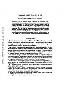
Speedup against Input Data Size 140
120
128 Proc s 64 Proc s 32 Proc s
Speedup, S(p)
100
16 Proc s 8 Proc s
80
60
4 Proc s
40
20
0 1024x1024
2048 x 2048
4096 x 4096
8192 x 8192
Input Data Dimension (MxN) 4 Proc s
8 Proc s
16 Proc s
32 Proc s
64 Proc s
128 Proc s
Figure 5. Speedup for parallel RScaLAPACK’s sla.solve() over serial R’s solve() function for different sizes of input data.
6.1. The Speedup The speedup factor, S(p) calculated is a measure of relative performance between a multiprocessor system and a single processor system and calculated as follows: S(p) = Tserial / Tparallel(p) where Tserial is the execution time using one processor and Tparallel is the execution time using p processors. Figure 5 shows the speedups taken for different input data sizes using varying number of processors. Two important observations can be made from the figure. First, the RScaLAPACK library is scalable in terms of both the problem size and the number of processors. Specifically, a consistent increase in the speedup with the increase in the number of processors used in RScaLAPACK function execution can be observed; further the speedup increases with the increase in the input data size. The second observation from Figure 5 is that a degree of loss in the speed gain can be observed while using more number of processors for performing sla.solve() function on a smaller input data size. Though this is subtly evident in Figure 5, it can be distinctly observed in Figure 6 below.
7
Speedup against Number of Processors 128 116.07
110.96
112
106.26 98.73
Speedup factor, S(p)
96 83.33 80
64
59.00
51.38
47.16
46.82
48
48.53
48.39
41.18 32
27.28 24.89
16
11.31
12.17
20.88
20.59
6.51
5.57
17.00
16.79
4.12
4.35
0 0
16
32
48
64
80
96
112
128
Number of Processes, p 1024 x 1024
2048 x 2048
4096 x 4096
8192 x 8192
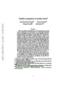
Figure 6. Speedup factor for parallel RScaLAPACK’s sla.solve() over serial R’s solve() function for different number of processors. From Figure 6 we can also observe that the speedup while evaluating a matrix of input size 1024x1024 using 4 processors is more than that achieved using 128 processors. For the input matrix of size 2048x2048 the best gain is attained using 8 processors and, similarly, for the input matrix of size 4096x4096 the best gain is achieved using 32 processors. In each of the above cases, beyond a certain point a consistent reduction in the speedup factor is observed for small size matrices, even if the number of processors used for the parallel computation is increased. This is the point where communication cost becomes significant when compared to the computational cost. Till this point even though there is a communication overhead its significance is meager when compared to the computational requirement. Figure 6 serves as a good benchmark for sla.solve() function, where given the size of input data, the user can use an optimum number of processors to take the maximum benefit from the underlying parallel algorithm provided by ScaLAPACK. 6.2. The Percentage Overhead We define the overhead O(p) that is induced by the Parallel Agent and the p, Spawned Processes in the R environment as follows: O(p) = [RScaLAPACK(p) – ScaLAPACK(p) / RScaLAPACK(p)] x 100 where RScaLAPACK(p) is the total function execution time using RScaLAPACK function in R and ScaLAPACK(p) is the ScaLAPACK function execution time. The overhead induced by the R environment and the Parallel Agent corresponds to the functionality of spawning p processes, distribution of the input data among these processes, and collection and
8
aggregation of the results from the spawned processes. The ScaLAPACK function execution part corresponds to the combined functionality of receiving input data chunk by each process, performing the computation using the ScaLAPACK function, and sending the result pieces to the Parallel Agent. Figure 7 shows the percentage overhead induced by the Parallel Agent for varying number of processes and input data sizes. Some distinct observations can be made from Figure 7, like the overhead is high when the input data size is small. As the input data size increases the percentage overhead drops significantly from almost 25% to 5%. This behavior is expected since the cost of performing ScaLAPACK computation on input data increases with the increase in the input data size, while the input distribution and the result collection cost reduces comparatively. Hence, we can conclude that the RScaLAPACK function usage is more efficient for the large input data size. Further, during our performance runs it was observed that for large input data matrices of dimensions 16384 x 16384 double precision data types, R failed to execute the solve() function, where RScaLAPACK sla.solve() succeeded to return expected result. This behavior of the system can be attributed to the design of RScaLAPACK, where the actual computations are performed outside the R environment.
Percentage Overhead induced by R environment and Parallel Agent 30
25
25.19
% Overhead, O(p)
24.76
23.88
20 17.24
15.51
14.46
15
10.42
10.38 10
7.96
10.03
9.61
5 4.74 0 4
64
128
Number of Processors, p 1024X1024
2048X2048
4096X4096
8192X8192
Figure 7: Percentage overhead induced by R environment and the Parallel Agent.
7. Conclusion and Future Work In this paper we presented the RScaLAPACK library to enable an R user to perform time efficient analysis on a large data set, using the high-performance ScaLAPACK library routines, while maintaining the same ease in the function usage. We have discussed the system design, usage and the performance characteristics of one of the RScaLAPACK functions (sla.solve). Through the graphs from the performance runs a high speedup in computation was observed while using RScaLAPACK functions.
9
Currently, no package or add-on library to R comparable to RScaLAPACK is found. The current function support provided by RScaLAPACK deals with the double precision data-type alone. Additional support for various data-types and more capabilities shall be added to the package in the near future. Continuing our effort on providing easy-to-use parallel solutions for data analysis packages like R, we are currently working on another R package called task-pR [23]. It achieves parallelism by performing out-of-order execution of R tasks. With its intelligent scheduling, the package is able to achieve significant improvement in data analysis times for certain types of R tasks. Work is also underway on another R package called PMatrix. It extends RScaLAPACK’s functionalities to include other matrix operations like matrix multiplication, matrix norm, etc., supports different matrix types, like symmetric, triangular, etc. of various data types like real, complex, and integer. Acknowledgments
This work is performed as part of the Scientific Data Management Center s Scientific Discovery through (http://sdmcenter.lbl.gov) under the Department of Energy' Advanced Computing (DOE SciDAC) program (http://www.scidac.org). The work is supported by the Office of Computational and Technology Research, Division of Mathematical, Information, and Computational Sciences, of the U.S. Department of Energy. We gratefully acknowledge the Center for Computational Science of Oak Ridge National Laboratory for giving access to Opteron and SGI Altix clusters for performing benchmarks. We are thankful to the development teams of the following Open Source software: R, ScaLAPACK, LAM-MPI, PVM, and MPI2. References [1] R. Choy and A. Edelman. “Parallel Matlab: Doing it right”, Nov 2003, http://wwwmath.mit.edu/~edelman/homepage/papers/pmatlab.pdf [2] A. Trefethen, V. Menon, "MultiMATLAB: integrating MATLAB with high-performance parallel computing", Proceedings of the 1997 ACM/IEEE conference on Supercomputing, Pages: 1 - 18, ISBN:0-89791-985-8, San Jose, CA, 1997 [3] R Development Core Team. “An Introduction to R.” June 2004, http://www.r-project.org [4] R Development Core Team. “Writing R Extensions.” June 2004, http://cran.r-project.org/manuals.html [5] H. Yu. “The rmpi package”, 2004, http://cran.r-project.org/doc/packages/Rmpi.pdf [6] N. Li and A. Rossini, “The rpvm package”, 2004, http://cran.r-project.org/doc/packages/rpvm.pdf [7] N. Li, H. Sevicikova, L. Tierney, A. Rossini. “The snow package”, 2004, http://cran.rproject.org/doc/packages/snow.pdf [8] L. Blackford, J. Choi, A. Cleary, E. D' Azevodo, J. Demmel, I. Dhillon, J. Dongarra, S. Hammarling, G. Henry, A. Petitet, K. Stanley, D. Walker, and R.C. Whaley. “ScaLAPACK User's Guide.” Society for Industrial and Applied Mathematics, 1997, http://www.netlib.org/scalapack/slug/ [9] J. Choi, J. Dongarra, L. Ostrouchov, A. Petitet, D. Walker and R. Whaley, “Design and Implementation of the ScaLAPACK LU, QR, and Cholesky factorization routines.”, Scientific Programming, 5(3):173-184, Fall 1996, http://citeseer.ist.psu.edu/article/choi96design.html
10
[10] E. Anderson, Z. Bai, C. Bischof, J. Demmel, J. Dongarra, J. Du Croz, A. Greenbaum, S. Hammarling, A. McKenney, S. Ostrouchov, and D. Sorensen. “LAPACK Users' Guide”, Second Edition. SIAM, Philadelphia, PA, 1995. [11] I. Jolliffe, “Principal Component Analysis”. New York: Springer-Verlag, 1986. [12] A. Geist, A. Beguelin, J. Dongarra, W. Jiang, R. Manchek and V. Sunderam “PVM: Parallel Virtual Machine A User’s Guide and Tutorial for Networked Parallel Computing”. The MIT Press, 1994. [13] W. Gropp. E. Lusk, and A. Skjellum. “Using MPI: Portable Programming with Message Passing Interface - 2nd edition”. The MIT Press, 1999, http://www-unix.mcs.anl.gov/mpi/usingmpi [14] P. Pacheo. “Parallel Programming with MPI”, Morgan Kaufmann Publishers Inc., 1997. [15] W. Gropp, E. Lusk, and R. Thakur. “Using MPI-2: Advanced Features of the Message Passing Interface”. The MIT Press, 1999. [16] G. Burns, R. Daoud and J. Vaigl, “LAM: An Open Cluster Environment for MPI”. In Proceedings of Supercomputing Symposium, pages 379-386, 1994, http://www.lam-mpi.org/download/files/lampapers.tar.gz [17] J. Squyres and A. Lumsdaine. “A Component Architecture for LAM/MPI”. In Proceedings, 10th European PVM/MPI Users'Group Meeting, number 2840 in Lecture Notes in Computer Science, pages 379-387, Venice, Italy, September / October 2003. Springer-Verlag. [18] Statistical Sciences Inc. "S-PLUS Reference Manual", 1991. [19] J. Dongarra and R. Whaley. “A user's guide to BLACS v1.0”. Technical Report CD-95-281, Department of Computer Science, University of Tennessee, 1995. [20] C. Whaley. “Using BLACS and MPI in ScaLAPACK”, Nov 1995, http://citeseer.ist.psu.edu/67272.html [21] R. Whaley. “Outstanding issues in the MPIBLACS”, Nov 1997, http://citeseer.ist.psu.edu/whaley95outstanding.html [22] J. Choi, J. Dongarra, and D. Walker, “PB-BLAS: A Set of Parallel Block Basic Linear Algebra Subroutines”, Proceedings of Scalable High Performance Computing Conference (Knoxville, TN), pp. 534-541, IEEE Computer Society Press, May 23-25, 1994. [23] D. Bauer, S. Yoginath, N. Samatova, G. Kora, A. Geist. “Task-pR: High-Performance Statistical Computing via Task-enabled Parallelism in R”
11