Parallel Computation of Pseudospectra using Transfer ... - CiteSeerX

Parallel Computation of Pseudospectra using Transfer Functions on a MATLAB-MPI Cluster Platform C. Bekas1 , E. Kokiopoulou1 , E. Gallopoulos1 , and V. Simoncini2 1

Computer Engineering and Informatics Department University of Patras, Greece [knb,exk,statis]@hpclab.ceid.upatras.gr 2 Mathematics Department University of Bologna, Italy [email protected]

Abstract. One of the most expensive problems in numerical linear algebra is the computation of the -pseudospectrum of matrices, that is, the locus of eigenvalues of all matrices of the form A + E, where the norm of E is bounded by . Several research efforts have been attempting to make the problem tractable by means of better algorithms and utilization of all possible computational resources. One common goal of these efforts is to bring to users the power to extract pseudospectrum information from their applications, on the computational environments they generally use, at a cost that is sufficiently low to render these computations routine. To this end, we investigate a scheme based on i) iterative methods for computing pseudospectra via approximations of the resolvent norm, with ii) a computational platform based on a cluster of PCs and iii) a programming environment based on MATLAB enhanced with MPI functionality and show that it can achieve high performance for problems of significant size.

1 Introduction and motivation Let A ∈ Cn×n have singular value decomposition (SVD) A = U ΣV ∗ , and let Λ(A) be the set of eigenvalues of A. The −pseudospectrum ˏ (A) (pseudospectrum for short) of a matrix is the locus of eigenvalues of Λ(A+E), for all possible E such that kEk ≤  for given  and norm. When A is normal (i.e. satisfies the relation AA∗ = A∗ A), the pseudospectral regions are readily computed as the union of the disks of radius  surrounding each eigenvalue of A. The pseudospectrum becomes of interest when A is nonnormal see [1], references therein and [2] for a package for pseudospectra computation using PVM. An important barrier in providing pseudospectral information routinely is the expense involved in their calculation. In the sequel we use the 2-norm for matrices and vectors, R(z) = (A − zI)−1 is the resolvent of A and ek the k th standard unit vector. Also s(x, y) := σmin (xI + iyI − A), herein written compactly as s(z) for z = x + iy, is the minimum singular value of matrix zI − A. Two equivalent definitions of the −pseudospectrum are ˏ (A) = {z ∈ C : σmin (A − zI) ≤ } = {z ∈ C : kR(z)k ≥

1 }. 

(1)

Relations (1) immediately suggest an algorithm, referred to as GRID, for the computation of ˏ (A) that consists of the following steps: i) Define grid Ωh on a region of the complex plane that contains ˏ (A). ii) Compute s(zh ) := σmin (zh I − A) or R(zh ), ∀zh ∈ Ωh . iii) Plot -contours of s(z) or R(z). GRID’s cost is modeled as CGRID = |Ωh | × Cσmin ,

(2)

where |Ωh | is the number of nodes of the mesh and Cσmin is the average cost of computing σmin . GRID is simple, robust and embarassingly parallel, since the computations of s(zh ) are completely decoupled between gridpoints. As cost formula (2) reveals, its cost increases rapidly with the size of the matrix and the number of gridpoints in Ωh . For example, using MATLAB version 6.1, the LAPACK 3.0 based svd function takes 19 sec to compute the SVD of a 1000 × 1000 matrix on a Pentium-III at 866 MHz. Computing the pseudospectrum on a 50 × 50 mesh would take almost 13 hours or about 7, if A is real and one use the fact that then, the pseudospectrum is symmetric with respect to the real axis. Exploiting the embarassingly parallel nature of the algorithm, it would take over 150 such processors to bring the time down to 5 min (or 2.5, in case of real A). As an indication of the state of affairs when iterative methods are used, MATLAB’s svds (based on ARPACK) on the same machine required almost 68 sec to compute s(z) for Harwell-Boeing matrix e30r0100 (order n = 9661, nnz = 306002 non-zero elements) and random z; furthermore, iterative methods over domains entail interesting load balancing issues; cf. [3, 4]. The above underline the fact that computing pseudospectra presents a formidable computational challenge since typical matrix sizes in applications can reach the order of hundreds of thousands. Cost formula (2) suggests that we can reduce the complexity of the calculation by domain-based methods, that seek to reduce the number of gridpoints where s(z) must be computed, and matrix-based methods, that target at reducing the cost of evaluating s(z). Given the complexity of the problem, it also becomes necessary that we use any advances in high performance computing at our disposal. All of the above approaches are the subject of current research.3 Therefore, if the pseudospectrum is to become a practical tool, we must bring it to the users on the computational environments they generally use, at an overall cost that is sufficiently low to render these computations routine. Here we present our efforts towards this target and contribute a strategy that combines: Parallel computing on clusters of PCs for high performance at low cost, communication using MPI-like calls, and programming using MATLAB, for rapid prototyping over high quality libraries with a very popular system. Central to our strategy is the Cornell Multitasking Toolbox for MATLAB (CMTM) ([5]) that enhances MATLAB with MPI functionality [6]. In the context of our efforts so far, we follow here the mathematical foundations of the “transfer function framework” described in [7]. Some first results, relating the performance of the transfer function framework on an 8 processor Origin-2000 ccNUMA system were presented in [8]. In [3], we described the first use of the CMTM system in the context of domain-based algorithms developed by our group as well as some load balancing issues that arise in the context of domain and matrix methods. In this paper, we extend our efforts related to the iterative computation of pseudospectra using the transfer function framework. 3

See also the site URL http://web.comlab.ox.ac.uk/projects/pseudospectra.

Table 1. Available CMTM commands (version 0.82) (actual commands prefixed with MMPI ). Abort, Barrier, Bcast, Comm dup, Comm free, Comm rank Comm size, Comm split, Gather, Iprobe, Irecv, Recv Reduce, Scatter, Scatterv, Send, Testany, Wtime

1.1

Computational environment

As a representative of the kind of computational cluster that many users will not have much difficulty in utilizing, in this paper we employ up to 8 uniprocessor Pentium-III @ 933MHz PCs, running Windows 2000, with 256KB cache and 256MB memory, connected using a fast Ethernet switch. We use MATLAB (v. 6.1) due to the high quality of its numerics and interface characteristics as well as its widespread use in the scientific community. The question arises, then, how to use MATLAB to solve problems such as the pseudospectrum computation in parallel? We can, for example translate MATLAB programs into source code for high performance compilers e.g. [9], or use MATLAB as interface for calls to distributed numerical libraries e.g. [10]. Another approach is to use multiple, independent MATLAB sessions with software to coordinate data exchange. This latter approach is followed in the “Cornell Multitasking Toolbox for MATLAB” [5], a descendant of the MultiMATLAB package [11]. CMTM enables multiple copies of MATLAB to run simultaneously and to exchange data arrays via MPI-like calls. CMTM provides easy-to-use MPI-like calls of the form A = MMPI Bcast(A); Each MMPI function is a MATLAB mex file, linked as a DLL with a commercial version of MPI, MPI/Pro v. 1.5, see [12]. Like MATLAB, CMTM functions take as arguments arrays. As the above broadcast command shows, CMTM calls are simpler than their MPI counterparts. The particular command is executed by all nodes; the system automatically distinguishes whether a node is a sender or a receiver and performs the communication. Similar are the calls to other communication procedures such as blocking send-receive and reduction clauses. For example, in order to compute a dot product of two vectors x and y that are distributed among the processors, all nodes execute the call MMPI Reduce(x’*y, MPI ADD); Each node performs the local dot product and then the system accumulates all local sub-products to a root node. Table 1 lists the commands available in the current version of CMTM. Notice the absence of the MPI ALL type commands (e.g. Allreduce, Allgather). Whenever these commands are needed, we simulate them, e.g. using reduce or gather followed by broadcast.

Baseline measurements In order to better appreciate the results for our main algorithm, we provide some baseline measurements for a few indicative collective communication operations on our computational cluster. We note that for all experiments in this work the cluster was in single user mode. Table 2 contains the measured timings with varying number of processors and problem sizes when using CMTM to broadcast vectors and also to reduce by summation. As expected, MMPI Reduce is always more time consuming than MMPI Bcast, while both take longer as the cluster size increases.

Table 2. Timings (in sec) for broadcasting and reducing summation of vectors of size 40000:20000:100000 using CMTM on p = 2, 4, 8 processors. MMPI Bcast MMPI Reduce p 40000 60000 80000 100000 40000 60000 80000 100000 2 0.03 0.05 0.06 0.08 0.05 0.05 0.06 0.081 4 0.07 0.09 0.12 0.15 0.09 0.13 0.13 0.16 8 0.09 0.13 0.17 0.22 0.13 0.15 0.19 0.24

2

The transfer function framework

An early, interesting idea for the economical approximation of the pseudospectrum, presented in [13], was to use Krylov methods and obtain approximations to σmin (zI − A), from σmin (zI − H), where H was either the square or the rectangular upper Hessenberg matrix that is obtained during the Arnoldi iteration and I is the identity matrix or a section thereof to conform in size with H. A practical advantage of this approach is that, whatever the number of gridpoints, it requires only one (expensive) reduction of A to upper Hessenberg form. It still requires, however, the (independent) computations of σmin (zh I − H), for every gridpoint zh , since, unlike eigenvalues singular values do not respect the shift property, i.e. in general, σ(zI − A) 6= z − σ(A). The above approach was further refined in [14]. Let now D∗ , E be full rank - typically long and thin - matrices, of row dimension n. Matrix Gz (A, E, D) := DR(z)E is called in the literature transfer function. It was shown in [7] that the transfer function provides a useful framework for describing existing and defining new methods for computing ∗ and pseudospectra. The central method in [7] was based on the selection D = Wm E = Wm+1 , where Wm = [w1 , . . . , wm ] denotes the orthonormal basis for the Krylov subspace Km (A, w1 ) constructed by the Arnoldi iteration, so that AWm = Wm Hm,m + hm+1,m wm+1 e> m,

(3)

where Hm,m is the square upper Hessenberg matrix consisting of the first m rows of Hm+1,m . We note that Wm+1 = [Wm , wm+1 ] and Hm+1,m = [Hm,m ; hm+1,m e> m ]. We will be referring to m as the “transfer function dimension” and will be writing ∗ Gz,m (A) for Gz (A, Wm+1 , Wm ). With the afore-mentioned selection for D and E, for ∗ large enough m we have kR(z)k ≈ kGz (A, Wm+1 , Wm )k, which provides an approximation to kR(z)k that improves monotonically with m and would be used in the sequel to construct the pseudospectrum based on relation (1); cf. [7]. Even though computa∗ ∗ (A − zI)−1 Wm+1 appears to require solving m + 1 tion of Gz (A, Wm+1 , Wm ) = Wm linear systems of size n, a trick allows us to reduce the number of (large) linear systems to one because > Gz,m (A) = [(I˜ − hm+1,m φz em )(Hm,m − zI)−1 , φz )],

(4)

∗ where φz = Wm (A − zI)−1 wm+1 ; cf. [7]. Therefore, in order to compute kGz,m (A)k we have to solve a single (large) linear system of size n for each shift z; furthermore,

Table 3. Arnoldi performance (in sec) for p = 1 to 8 processors using CGS, MGS and CGS with reorthogonalization on random sparse matrices of size n. Arnoldi p \ n 40000 60000 80000 100000 p \ n 40000 60000 80000 100000 CGS 1 328 512 1716 5885 2 150 241 340 440 MGS 362 560 1453 3126 172 265 365 476 CGSo 389 606 1780 6962 181 289 405 522 CGS 4 80 126 179 235 8 53 80 113 143 MGS 129 158 209 268 92 125 188 201 CGSo 101 150 211 275 64 97 135 164

the right hand side, wm+1 , remains the same for each shift, something that will be exploited by the iterative solver (cf. the next section). We also need to solve m Hessenberg systems of size m, and to compute the norm of Gz,m (A). We discuss the actual parallel implementation of this approach for our cluster environment in Section 2.1. The Arnoldi iteration As with most modern iterative schemes, the effective implementation of the transfer function methodology uses the Arnoldi iteration, via an implementation of relation (3), as a computational kernel, to create an orthogonal basis for the Krylov subspace [15]. We organize the iteration around a row-wise partition of the data: Each processor is assigned a number of rows of A and V . At step j, we store the entire V (:, j) that must be orthogonalized into each processor. This requires a broadcast, at some point during the iteration, but allows thereafter the matrix-vector multiplication to take place locally on each processor. Due to lack of space we do not go into further details but tabulate, in Table 3, results from experiments on our cluster and programming environment with three different types of Arnoldi iteration: CGS-Arnoldi, MGS-Arnoldi and CGSo-Arnoldi, where the first is based on classical Gram-Schmidt (GS) orthogonalization, the next on modified GS and the last on classical GS with selective reorthogonalization. Notice the superlinear speedup for the larger matrices due to the disribution of the large Krylov bases. The random sparse matrices were created using the MATLAB’s built-in function sprand(n,n,p) with p equal to 3e − 4. 2.1

TRGRID: GRID with transfer functions

The property that renders Krylov type linear solvers particularly suitable in the context of the transfer function framework for pseudospectra, in particular formula (4), is the shift invariance of Krylov subspaces, i.e. the fact that Kd (A, w1 ) = Kd (A − zI, w1 ) for any z. This means that we can reuse the same basis that we build for Kd (A, w1 ), say, to solve linear systems with “shifted” matrices, e.g. A − zI; see for example [16]. Since our interest is in nonnormal matrices, we used GMRES as the linear solver. The pseudocode for our parallel algorithm is listed in Table 4. Remember that after completing the (parallel) Arnoldi iterations (Table 4, line 1), ˆ are diswith the row distribution described earlier, the rows of the bases W and W tributed among the cluster nodes. For the sake of economy in notation we use the same

Table 4. Pseudocode for the parallel TRGRID algorithm for the CMTM environment Parallel TRGRID (* Input *) Points zi , i = 1, ..., M , vector w1 with kw1 k = 1, scalars m, d. 1. All nodes work on two parallel Arnoldi iterations [Wm+1 , Hm+1,m ] ← arnoldi (A, w1 , m) ˆ d+1 , Fd+1,d ] ← arnoldi(A, wm+1 , d) [W ˆ d+1 Each node has some rows of Wm+1 , W Node zero distributes the M gridpoints so that processor pr id holds points in the M/p-sized set I(pr id) 2. for i ∈ I(pr id) Y (:, i) = argminy {k(Fd+1,d − zi I˜d )y − e1 k} 3. 4. end 5. Node zero gathers matrix Y and broadcasts it back ∗ ˆ 6. Each node performs local multiplication φz,i = Wm Wd Y 7. Node zero collects Φz =Reduce(φz ,SUM) 8. Node zero distributes back the columns of Φz 9. for i ∈ I(pr id) > )(Hm,m − zi I)−1 10. Di = (I˜ − hm+1,m Φz (:, i)em 11. kGzi (A)k = k[Di , φzi ]k 12. end 13. Node zero gathers approximations of 1/s(zi )

symbolism when we deal with local computations too, while in reality we are referˆ . Each processor (see lines 2-4, 9-12) ring only to a subset of the rows of W and W works on M/p gridpoints (we have assumed that p exactly divides M ). In line 3, each node computes its share of the columns of matrix Y . For the next steps, in order for the local φz to be computed, all processors must access the whole Y , hence all-to-all type communication is needed. In lines 9-12 each processor works on its share of gridpoints and columns of matrix Φz . Finally, processor zero gathers the approximations M of {1/s(zi )}i=1 . What remains to clarify is the computation of φz,i and Φz (lines 6ˆ i Y , where Wi and W ˆ i , i = 0..., P − 1 are the subsets of 7). We have φz,i = Wi∗ W ˆ that each node privately owns. Then, contiguous rows of the basis matrices W and W PP −1 Φz = φ and we use reducing summation to compute Φz in parallel, since z,i i=0 CMTM allows reduction processes to work on matrices as well as scalars. It is worth noting that the preferred order used when applying to implement the two matrix-matrix ˆ i and on multiplications of line 6 depends on the dimensions of the local matrices Wi , W the column dimension of Y and could be decided at run time. In our experiments, we assumed that the Krylov dimensions m, d were much smaller than the size of the matrix, n, and the grid, M . TRGRID consists of two parts. The first part (line 1) consists of the Arnoldi iterations used to obtain orthogonal bases for the Krylov subspaces used for the transfer function and for the solution of the size n system. In forthcoming work we detail techniques that exploit the common information present in the two bases ([8]). An important advantage of the method is that after the first part is completed and basis ma-

Table 5. Performance of parallel TRGRID gre 1107 pores 2 sprand(2000) sprand(4000) p 1 2 4 8 1 2 4 8 1 2 4 8 1 2 4 8 Time (sec) 174 76.2 36.2 18.7 340 155 76.3 38.1 244 118.8 59.3 31 501 245 123 63.9 Speedup - 2.3 4.8 9.3 - 2.2 4.5 8.9 - 2.1 4.1 7.87 - 2.04 4.1 7.84

0.8

1 0.8

0.6

0.6 0.4

0.4 0.2

0.2

0

0

−0.2 −0.2

−0.4 −0.4

−0.6 −0.6

−0.8 −1 −1

−0.5

0

0.5

1

−0.8 −2

−1.5

−1

−0.5

0

0.5

1

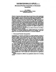
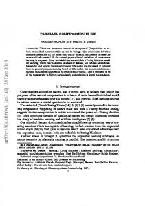
Fig. 1. Pseudospectrum contour ∂ˏ (A),  = 1e − 1 for gre 1107 (left) and pores 2 (right).

ˆ become available, we only need to repeat the second part, from line 2 trices W and W onwards to compute the pseudospectrum. Based on this property and given the previous results for Arnoldi we measure the performance of only the second part of TRGRID. A second observation is that the second TRGRID involves only dense linear algebra. Remember also that at the end of the first part, each processor has a copy of the upper Hessenberg matrices. Hence, we can use BLAS-3 to exploit the memory hierarchy of each processor. Furthermore, assuming that M ≥ p, the workload would be evenly divided amongst processors. Of course, the method is always subject to load imbalances due to systemic effects. However, since the second part of parallel TRGRID requires only limited communication, increased network traffic is not expected to have a significant effect on performance. Let us now investigate the performance of the main body of parallel TRGRID on our cluster’s nodes. We experimented with the HB-matrices gre 1107 (n = 1107, nnz = 5664) and pores 2 (n = 1124, nnz = 9613) scaled by 1e − 7, as well as with two random sparse matrices of size n = 2000 and 4000 with density p = 1e − 2. On the domain [−1.8, 1.8] × [−1.8, 1.8], we employed a 50 × 50 grid for the HB matrices and a 30 × 40 grid for the random matrices. Figure 1 illustrates the  = 0.1 contours for the two HB matrices. The Krylov dimensions were m = d = 75, 100, 120 and 150 respectively. Table 5 illustrates the performance results. In all cases, except for p = 8 for the random matrices we observe excellent, superlinear in most cases, (absolute) speedups due to the fact that the Krylov bases are distributed.

3

Conclusions

The widespread availability of the high quality numerics and interface of MATLAB together with an MPI-based parallel processing toolbox and the results shown in this

paper for matrix-based methods and in [3] for domain based methods, indicate that the computation of pseudospectra of large matrices is rapidly becoming accessible to everyday users who prefer to program in MATLAB and whose only hardware infrastructure is a PC cluster. Further work in progress includes the incorporation of these methods into a toolbox as well as the exploitation of multithreading, testing different forms of parallelism for MATLAB as well as the enhancement of the numerical infrastructure with lower level parallel computational kernels, e.g. SCALAPACK-like. We are also working on several numerical issues that arise during the combination of the transfer function approach with domain based methods so as to permit even more effective and robust implementations [8].

References 1. Trefethen, L.: Computation of pseudospectra. In: Acta Numerica 1999. Volume 8. Cambridge University Press (1999) 247–295 2. Braconnier, T.: Fvpspack: A Fortran and PVM package to compute the field of values and pseudospectra of large matrices. Numerical Analysis Report No. 293, Manchester Centre for Computational Mathematics, Manchester, England (1996) 3. Bekas, C., Kokiopoulou, E., Koutis, I., Gallopoulos, E.: Towards the effective parallel computation of matrix pseudospectra. In: Proc. 15th ACM Int’l. Conf. Supercomputing (ICS’01), Sorrento, Italy. (2001) 260–269 4. Mezher, D., Philippe, B.: Parallel computation of the pseudospectrum of large matrices. Parallel Computing 28 (2002) 199–221 5. Zollweg, J., Verma, A.: The Cornell Multitask Toolbox. Directory Services/Software/CMTM at URL http://www.tc.cornell.edu (2002) 6. Gropp, W., Lusk, E., Skjellum, A.: Using MPI: Portable Parallel Programming with the Message Programming Interface. second edn. MIT Press, Cambridge, MA (1999) 7. Simoncini, V., Gallopoulos, E.: Transfer functions and resolvent norm approximation of large matrices. Electronic Transactions on Numerical Analysis (ETNA) 7 (1998) 190–201 8. Bekas, C., Gallopoulos, E., Simoncini, V.: On the computational effectiveness of transfer function approximations to the matrix pseudospectrum. In: Proc. Copper Mountain Conf. Iterative Methods. (Apr. 2000) Full paper in preparation. 9. DeRose, L., et al.: FALCON: A MATLAB Interactive Restructuring Compiler. In C.-H. Huang, et al., ed.: Lecture Notes in Computer Science: Languages and Compilers for Parallel Computing. Springer-Verlag, New York (1995) 269–288 10. Casanova, H., Dongarra, J.: NetSolve: A network server for solving computational science problems. Int’l. J. Supercomput. Appl. and High Perf. Comput. 11 (1997) 212–223 11. Menon, V., Trefethen, A.: MultiMATLAB: Integrating MATLAB with high-performance parallel computing. In: Proc. Supercomputing’97. (1997) 12. MPI Software Technology: (MPI/Pro) http://www.mpi-softtech.com. 13. Toh, K.C., Trefethen, L.: Calculation of pseudospectra by the Arnoldi iteration. SIAM J. Sci. Comput. 17 (1996) 1–15 14. Wright, T., Trefethen, L.N.: Large-scale computation of pseudospectra using ARPACK and Eigs. SIAM J. Sci. Stat. Comput. 23 (2001) 591:605 15. Dongarra, J., Duff, I., Sorensen, D., van der Vorst, H.: Numerical Linear Algebra for HighPerformance Computers. SIAM (1998) 16. Frommer, A., Gl¨assner, U.: Restarted GMRES for shifted linear systems. SIAM J. Sci. Comput. 19 (1998) 15–26