147 neural network data preprocessing: is it necessary for ... - DergiPark

Akademik Araştırmalar ve Çalışmalar Dergisi Cilt: 9, Sayı: 17, Yıl: 2017

Journal of Academic Researches and Studies Vol: 9, No: 17, Year: 2017

Geliş Tarihi / Received: 18.07.2017 Kabul Tarihi / Accepted: 20.09.2017

Sayfa / pp: 147-154

NEURAL NETWORK DATA PREPROCESSING: IS IT NECESSARY FOR TIME SERIES FORECASTING? *** YAPAY SİNİR AĞLARI VERİ ÖN İŞLEMESİ: ZAMAN SERİSİ TAHMİNLEMESİ İÇİN GEREKLİ MİDİR? Assist. Prof. Dr. Hakan PABUÇCU Bayburt University Faculty of Economics and Administrative Sciences Department of Business [email protected]

Abstract Neural networks (NNs) are a commonly used method to solve the time series-forecasting problem. NNs have some advantages compared with traditional forecasting models, such as auto regressive moving average or auto regressive integrated moving average. NNs do not need to have any statistical assumption like normal distribution. However, data preprocessing, normalization, trend adjusting, seasonal adjusting, or both differencing can introduce better results in some studies. In this study, we have tried to investigate whether data preprocessing methods are useful for time series data, which contains trend, seasonality or unit root. For this purpose, we collected the real time series data belonging to monthly or quarterly observations and used nonlinear autoregressive (NAR) and multilayer perceptron (MLP) models. Although we obtained significant differences between data preprocessing methods, the structure of MLP with differenced variable produced the worst results. Keywords: Data preprocessing, neural networks, time series forecasting

Öz Yapay sinir ağları zaman serisi tahmini problemlerinin çözümünde sıklıkla kullanılan modellerdir. ARMA veya ARIMA gibi geleneksel zaman serisi tahmin modelleri ile karşılaştırıldıklarında da bazı avantajlara sahiptirler. Sinir ağları normal dağılıma uygunluk gibi değişkenlerin sağlaması gereken bazı istatistiksel varsayımların sağlanmasını gerektirmez. Bununla birlikte normalizasyon, trenden arındırma veya mevsimsel düzeltme gibi bazı veri ön işleme uygulamaları ile daha iyi sonuçların üretildiği de bazı çalışmalarda görülmektedir. Bu çalışmada, trend, mevsimsellik ve birim kök içeren zaman serilerine uygulanan veri ön işleme uygulamalarının tahmin sonuçlarına etkileri araştırılmıştır. Bu amaçla, bazı değişkenlere ait aylık ve çeyreklik veriler kullanılarak doğrusal olmayan oto regresif (NAR) ve çok katmanlı algılayıcı (MLP) modellerinin tahmin performansları araştırılmıştır. Sonuçlara göre veri ön işleme uygulamaları arasında önemli farklılıklar tespit edilmekle birlikte, fark serileri ile oluşturulan MLP modellerinin en kötü sonuçları ürettiği açık bir şekilde görülmüştür. Anahtar Kelimeler: Veri ön işleme, sinir ağları, zaman serisi tahmini

147


1.


INTRODUCTION

Many economic time series contain seasonality and trend variations. Generally, seasonal effects emerge in monthly or quarterly data. Seasonal effects could not emerge explicitly in annual data because they are the sum of weekly, monthly, or quarterly data. Seasonality is a recurrent effect that stems from the weather, holidays or any other periodic reason (Hylleberg, 1992). Forecasting accuracy is very important for seasonal and trend time series data to obtain efficient decisions in many fields (Makridakis et al., 1982). A large number of seasonal adjustment methods have been developed to eliminate the seasonal effect. Although eliminating the seasonal effect is very important for the accuracy of the results, it can lead to undesirable nonlinear features in univariate time series (Ghysels, Granger, & Siklos, 1996). As reported in Hylleberg (1992) seasonal effects can be not constant and so may change over time. In some time, series the seasonal and nonseasonal parts of the series can be dependent and, therefore, not divisible. Another effect on the data is the trending variation, which affects the forecasting accuracy of many traditional methods. The accuracy level of forecasting reduces because of the merging of these two effects. If the series contains trend variations it is called nonstationary. To obtain stationarity in Box-Jenkins methodology the process of differencing is applied for time series forecasting. However, this method is not always appropriate to model trends. Many different methods can be used to obtain nonstationary time series, such as a linear trend adjusting. If the series has a deterministic trend (i.e. trend stationary series), then a linear or polynomial trend model can be used. However, if it has a stochastic trend or unit root (difference stationary series), then a random walk model can be more convenient (Zhang & Qi, 2005). Several tests have been used to detect the unit root, such as Augmented Dickey Fuller or Philips Perron unit root test. An artificial neural network (NN) is a universal model that can be used to capture the linear or nonlinear relationship between variables and it has recently been widely used in financial and economic time series with seasonal and trend variations. NNs have been a perfect competitor with recent development and application in this field. There is no particular assumption while modelling with NNs. This feature is one of the most important advantage of NNs because it can help to solve real life problems (Zhang & Qi, 2005). Because of NNs natural structure, they can be used directly to forecast seasonal and trend time series. Some related literature supports this assumption. For example, Gorr (1994) stated that NNs could explore a concurrent nonlinear trend and seasonal effects. Sharda and Patil (1992) pointed out that NNs have an ability to model seasonality and, therefore, seasonal adjustment is not necessary for forecasting. Zhang and Qi ( 2005) pointed out that there have been dramatic reductions between original and preprocessed data errors. The last study that is related to the data preprocessing effect that we have been able to find was published in 2005. Consequently, we decided to study data preprocessing effects for the learning process and forecasting performance of NNs. The purpose of this paper is to investigate how the NNs could provide forecasts that are more accurate. The research question is whether data preprocessing is necessary. In addition, do NNs have the ability to model seasonal and trend time series directly? To test our hypothesis, we used the data from the United States monthly or quarterly figures that contain trend seasonal effects. 2.

EMPIRICAL METHODOLOGY

In this study, we consider the effect of data preprocessing methods on the learning and forecasting process for the NNs. The research questions are: i.

Do NNs have the ability to forecast trend and seasonal time series directly?

ii.

Is data preprocessing necessary to generate more accurate results?

iii. Are there any significant differences between the multilayer perceptron (MLP) and nonlinear autoregressive (NAR) models? To test these research questions, we used data that includes monthly or quarterly observations covering several different periods and fields, as shown in Table 1. The main reason for choosing these

148



series is that they contain trend and seasonal effects, depending on their frequency. Therefore, we are able to examine the effect of trend adjusting, seasonal adjusting, or both. The data was collected from the Federal Reserve Bank of St. Louis. Table 1. Variable Definition Variable Industrial Production Industrial Production House Price Index House Price Index Manufacturer Trade Balance

Frequency Monthly Quarterly Monthly Quarterly Monthly Quarterly

Code MIPCON QIPCON MHPI QHPI MNFCT TB

Period 1939M1-2016M11 1939M1-2016M11 1991M1-2016M10 1991M1-2016M10 1992M1-2016M10 1960M1-2014M10

We applied the following four data preprocessing to the original time series: i. trend adjustment (deterministic trend); ii. seasonal adjustment; iii. trend and seasonal adjustment; and iv. differencing (stochastic trend). We obtain the trend adjustment series by fitting a linear trend and extracting the forecasted trend (deterministic) from the original series. This is called seasonal adjustment or deseasonalization is made by using X-12-ARIMA seasonal adjustment methodology (Findley, Monsell, Bell, Otto, & Chen, 1998). We coded the data as original (OR), trend adjusted (TA), seasonally adjusted (SA), trend and seasonally adjusted (TSA), and differenced (DIF). NNs are a strong model to solve real problems in pattern recognition, time series forecasting and to construct the control or expert system. NNs can be considered to be a highly simplified model structure of the biological neuron (Yegnanarayana, 2005). NNs have the ability to learn from the last samples and they can forecast any linear or nonlinear relationship with high accuracy. Although many NN structures have been developed, MLP is the most commonly used for forecasting. MLP consist of input, hidden, and output nodes. The output nodes produce the forecast value while the input nodes receive the incoming signal from the out world. The network must have one or more hidden layers, with appropriate nonlinear activation function that help to increase the ability of learning (Öztemel, 2006). The model can be written as in Eq. 1: ∑

(∑

)

(1)

here are the number input and hidden nodes, respectively. function such as the logistic in Eq. 2:

is the sigmoidal activation (2)

here

is output of the neuron,

is weighted sum of all synaptic inputs with the bias.

The weight vector to output is and the weight vector to hidden nodes is . Eq. 3 is an identical form of nonlinear AR model. Another model to forecast time series that is identical to the MLP model that was presented in Eq. 1 is a nonlinear auto regressive (NAR) NN model (Hornik, Stinchcombe, & White, 1989). NAR is a special form of feedforward NNs for forecasting only time series while considering the autocorrelation between the error terms. The future values of dependent (output) variables are only forecast by using past values that are shown in series in Eq. 3: (

).

(3)

In this study, we used both the standard feedforward MLP and NAR models, and we presented the statistics related to both models to compare their performance. Logistic activation function was used for hidden nodes and linear function was used for the output node. Bias terms for hidden and output layers and Levenberg-Marquardt learning algorithm were used. Matlab 2011b-NN toolbox was used to solve the problems. To determine the best structure of the NN models, following Bishop (1995) and Ripley (1996) the dataset was divided into the following three parts: training, validating and testing. The training set is used to estimate the parameters, a validating set is to choose the best

149



model between other estimated models, and a test set is to verify the model’s stability. To determine the best NN model for each dataset: the number of hidden neurons varied from 2 to 20, the number of lags varied from 4 to 36 for monthly data, and from 2 to 9 for quarterly data. We estimated the NAR model first and MLP model second to use the same number of lags for both models. We calculated the most commonly used error statistics root mean square error (RMSE), mean squared error (MSE) and mean absolute percentage error (MAPE) to compare the models’ performance. RMSE and MSE are absolute value and MAPE is a relative value statistic. The models’ performance can be directly compared because we have converted the network outputs to original values.

3.

EMPIRICAL FINDINGS

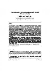
We estimated the NAR and MLP model for all of the datasets. Appendices A and B present the NAR and MLP modelling and forecasting error statistic, respectively. The datasets were divided into the following three parts: training, validating and testing. Dataset partitioning was randomly made and was 70%, 15% and 15%, respectively, for the three parts (i.e. training, validating, and testing). It is possible to make a lot of comments by using the performance measure. Initially, the NAR and MLP models can directly model the trend and seasonal time series. Figure 1 only presents the MAPE statistics for the training data. As can be seen in Figure 1 (for training dataset), the MAPE statistics that belong to the original series are generally upper than the preprocessed data. To make better and more accurate comparisons, we preferred the use the MAPE statistics because they are a relative measure. Similar results are found for valid RMSE and MSE statistics. Figure 1. MAPE statistics for NAR model training data

MIPCON

QHPI

MHPI

0,016 0,017 0,013 0,014 0,016

0,357 0,345 0,23 0,226 0,412

SA

0,663 0,284 0,311 0,22 0,59

QIPCON

TA

0,593 0,347 0,332 0,583 0,566

0,73 0,717 0,538 0,546 0,714

OR

2,008 2,503 1,623 1,92 2,36

NAR-MAPE-TRN

TB

MNFCT

The validation set is very important to evaluate the model’s performance. Figure 2 shows that the MAPE statistics that belong to the original series are generally upper than other preprocessed data. However, it is easy to observe that some preprocessed data, such as differenced, is sometimes upper than the others.

150



Figure 2. MAPE statistics for NAR model validating data NAR-MAPE-VAL TA

SA

0,785 0,521 0,545 0,721 0,658

1,559 0,259 0,803 0,052 0,792

0,77 0,627 0,542 0,476 0,544

QIPCON

MIPCON

QHPI

MHPI

0,019 0,011 0,008 0,008 0,018

0,857 0,8 0,659 0,582 0,925

5,8 5,25 4,824 5,842 6,557

OR

TB

MNFCT

The testing set that is out of sample for learning process reflects the stability of the network. As can be seen in Figure 3, the MAPE statistics have been reducing generally with data preprocessing. Generally, in the original series the MAPE statistics are upper than preprocessed data statistics. Only the trade balance model is different from the others. However, there is no certain evidence about the superiority of the data preprocessing methods relative to each other.

Figure 3. MAPE statistics for NAR model testing data

NAR-MAPE-TEST TA

SA

TSA

DIF

0,806 0,461 0,459 0,726 0,795

0,618 0,248 0,441 0,202 0,297

0,726 0,567 0,355 0,306 0,459

QIPCON

MIPCON

QHPI

MHPI

0,019 0,01 0,009 0,009 0,013

0,881 0,82 0,603 0,409 0,789

6,302 4,977 8,565 6,395 6,521

OR

TB

MNFCT

Second, we estimated the MLP model by using the optimal lag number, which comes from the NAR model. Figures 4 to 6 summarize the comparison of the models and MAPE statistics. Figure 4. MAPE statistics for MLP model training data

MLP-MAPE-TRN TA

SA

TSA

DIF

0,339 0,353 0,329 0,678 0,597

0,724 0,663 0,396 0,192 0,747

0,347 0,327 0,23 0,201 0,372

QIPCON

MIPCON

QHPI

MHPI

151

0,019 0,022 0,013 0,013 0,028

0,675 0,705 0,52 0,538 0,706

2,339 2,217 1,791 1,626 2,47

OR

TB

MNFCT



The data preprocessing methods, except difference, reduce the errors while using MLP. As seen in Figures 4 to 6, the MAPE statistics that belong to differenced models are generally upper than the original series and other preprocessed models. Therefore, it is possible to say that the difference extraction process is not useful for the MLP model. Trend and seasonal adjustment methods have in general reduced the error, as can be seen in Figures 4 to 6 or Appendix A and B. Figure 5. MAPE statistics for MLP model validating data

QIPCON

MIPCON

QHPI

MHPI

0,018 0,019 0,009 0,013 0,024

DIF

0,815 0,605 0,593 0,451 0,859

TSA

2,06 1,376 0,852 0,271 1,782

SA

0,547 0,548 0,531 0,717 0,711

TA

0,805 0,761 0,615 0,609 0,802

OR

6,796 5,957 4,057 6,753 7,257

MLP-MAPE-VAL

TB

MNFCT

If we examine the estimated models, the lower MAPE statistics belong to MNFCT while the upper one belongs to TB. Appendix A and B summarize that the MSE, RMSE, MAPE statistics belong to all of the estimated models. Figure 6. MAPE statistics for MLP model testing data

MLP-MAPE-TEST TA

SA

TSA

DIF

0,472 0,47 0,439 0,706 0,799

0,959 0,374 0,719 0,289 1,073

0,638 0,578 0,396 0,329 0,594

QIPCON

MIPCON

QHPI

MHPI

0,019 0,015 0,01 0,008 0,028

0,717 0,684 0,578 0,703 1,028

4,172

8,328

8,466 7,877 7,583

OR

TB

MNFCT

In this study, the results of NAR and MLP should be evaluated separately because they have some differences. We concluded that both models are generally able to directly forecast the trend and seasonal time series. The error statistics generally decrease after data preprocessing. It is also possible to see some differences based on the used data noise level. However, the general opinion is that the data preprocessing is useful to forecast trend and seasonal time series for the NAR model. The effect of data preprocessing is sometimes lower, sometimes upper. The type of data preprocessing method affects the forecasting performance of the NAR model. Seasonal adjustment has been identified as the most important method due to lower error statistics. Differencing has the lower effect on NAR modelling performance and forecasting ability. On the other hand, the MLP model also has the ability to directly forecast the trend and seasonal time series. Trend and seasonal adjustment are generally useful to increase the power of the model. However, the model with differenced series has upper error statistics, even when compared with the original series. Therefore, purifying the series from the stochastic trend is not useful for the performance of the MLP model. In brief, it is found that contrast to previous studies (Alon, Qi, & Sadowski, 2001; Hamzaçebi, 2008) the ANN and MLP model

152



produce more accurate results when using seasonally adjusted and trend adjusted data. The findings support the previous studies (Nelson, Hill, Remus, & O’Connor, 1999; Zhang & Kline, 2007; Zhang & Qi, 2005) with some little differences. It is thought that the differences are related to data set length, frequencies and used ANN model type. As a result of the study, it is not possible to say differencing is useful to improve the forecasting performance due to the loss of the information. The best two model structures for NAR and MLP are given in Table 2. Table 2. The Best Two Network Model Structure Model NAR

MLP

4.

Type of preprocessed O TA SA TSA DIF O TA SA TSA DIF

First MNFCT MNFCT MNFCT MNFCT MNFCT MNFCT MNFCT MNFCT MNFCT MNFCT

Optimal Lag 24 12 12 12 6 24 12 12 12 6

Hidden

Second

10 10 10 10 11 12 12 10 10 12

MHPI QHPI MHPI QHPI MHPI MIPCON MIPCON MIPCON MHPI MIPCON

Optimal Lag 24 12 12 12 6 36 36 36 12 18

Hidden 10 10 10 8 11 12 12 12 10 10

CONCLUSIONS

Data preprocessing is a very important phenomenon for many econometric, statistical, and mathematical analyses. Trend and seasonal adjustment are the two most commonly used methods. In this paper, we investigate the NN ability of modelling and forecasting seasonal and trend time series. We consider two types of trend variations: deterministic and stochastic. We obtain deterministic trend adjustment series by fitting a linear trend and extracting the forecasted trend from the original series. We obtain the stochastic trend by using a difference operator. The main research question is whether NN models provide more accurate results when data preprocessing performed. For this purpose, we got six real time series data, which have trend and seasonal variations. The results indicate that NNs have the ability to model and forecast trend and seasonal time series. However, data preprocessing is able to provide more accurate results. The models constructed by using differenced variable in MLP do not provide good results. Comparing the NAR and the MLP models—NAR generally provides more accurate results, although there is no clear distinction. The data preprocessing is useful for NNs but it is not possible to make a clear distinction between these methods. While sometimes a trend adjustment provides better results, sometimes a seasonal adjustment gives better results. Consequently, no clear distinction can be made. In addition, many time series studies on neural networks are available in the literature. The used data sets are not subjected to any preprocessing process since the work done is usually based on the assumption that neural networks do not require any assumptions. This study seems to be important for the research that will be done because it strengthens the belief that more accurate estimates can be obtained in time series problems by conducting the data preprocessing.

References ALON, I., QI, M. ve SADOWSKI, R. J. (2001). "Forecasting Aggregate Retail Sales", Journal of Retailing and Consumer Services, 8(3): 147–156. http://doi.org/http://dx.doi.org/10.1016/S0969-6989(00)00011-4 BISHOP, C. M. (1995). Neural Networks for Pattern Recognition, New York, NY: Oxford University Press. 153



FINDLEY, D. F., MONSELL, B. C., BELL, W. R., OTTO, M. C. ve CHEN, B.C. (1998). "New Capabilities and Methods of the X-12-ARIMA Seasonal-Adjustment Program", Journal of Business & Economic Statistics, 16(2): 127–152. http://doi.org/10.1080/07350015.1998.10524743 GHYSELS, E., GRANGER, C. W. J. ve SIKLOS, P. L. (1996). "Is Seasonal Adjustment a Linear or Nonlinear Data-Filtering Process?", Journal of Business & Economic Statistics, 14(3): 374–386. http://doi.org/10.1080/07350015.1996.10524663 GORR, W. L. (1994). "Editorial: Research Prospective on Neural Network Forecasting". International Journal of Forecasting, 10(1): 1–4. http://doi.org/http://dx.doi.org/10.1016/0169-2070(94)90044-2 HAMZAÇEBİ, C. (2008). "Improving artificial Neural Networks’ Performance in Seasonal Time Series Forecasting", Information Sciences, 178(23): 4550–4559. http://doi.org/http://dx.doi.org/10.1016/j.ins.2008.07.024 HORNIK, K., STINCHCOMBE, M. ve WHITE, H. (1989). "Multilayer Feedforward Networks are Universal Approximators", Neural Networks, 2(5): 359–366. http://doi.org/http://dx.doi.org/10.1016/0893-6080(89)90020-8 HYLLEBERG, S. (1992). Modelling Seasonality (1st ed.), Oxford: Oxford University Press. MAKRıDAKIS, S., ANDERSEN, A., CARBONE, R., FILDES, R., HIBON, M., LEWANDOWSKI, R., … WINKLER, R. (1982). "The Accuracy of Extrapolation (Time Series) Methods: Results of a Forecasting Competition", Journal of Forecasting, 1(2): 111–153. http://doi.org/10.1002/for.3980010202 NELSON, M., HILL, T., REMUS, W. ve O’CONNOR, M. (1999). "Time series Forecasting Using Neural Networks: Should the Data Be Deseasonalized First?", Journal of Forecasting, 18(5): 359–367. http://doi.org/10.1002/(SICI)1099131X(199909)18:53.0.CO;2-P ÖZTEMEL, E. (2006). Yapay Sinir Ağları (2nd ed.), İstanbul: Papatya Yayıncılık. RİPLEY, B. D. (1996). Pattern Recognition and http://doi.org/http://dx.doi.org/10.1017/cbo9780511812651

Neural

Networks.

SHARDA, R. ve PATIL, R. B. (1992). "Connectionist Approach to Time Series Prediction: An Empirical Test", Journal of Intelligent Manufacturing, 3(5): 317–323. http://doi.org/10.1007/BF01577272 YEGNANARAYANA, B. (2005). Artificial Neural Networks (11th ed.), New Delhi: Prentice-Hall of lndia Private Limited. ZHANG, G. P. ve KLINE, D. M. (2007). "Quarterly Time-Series Forecasting with Neural Networks", IEEE Transactions on Neural Networks, 18(6): 1800–1814. http://doi.org/10.1109/TNN.2007.896859 ZHANG, G. P. ve QI, M. (2005). "Neural Network Forecasting for Seasonal and Trend Time Series", European Journal of Operational Research, 160: 501–514. http://doi.org/10.1016/j.ejor.2003.08.037

154