(1991) 159 A Unified Approach to Dynamic Estimation* 1

INFORMATION

159

SCIENCES 57-58, 159-169 (1991)

A Unified Approach to Dynamic Estimation* ROBERT KALABA Departments of Electrical and Biomedical Engineering. Caiiforniu. Los Angeles, California 90089

Univbrsity

ofSouthern

LEIGH TESFATSION Departments of Economics Ames, Iowa 50011-1070

and Mathematics,

Iowa State University.

ABSTRACT Discrepancies between assumed dynamical models and observations are often handled by making further probabiIistic assumptions, a tactic which has both strengths and weaknesses. A re-examination of filtering and smoothing is conducted, and an alternative multicriteria approach, which is probability free, is advanced. This approach involves vector minimization as a key ingredient, and it specializes to the well-known Kalman. Viterbi. Larson-Peschon, and Swerling filters.

1. INTRODUCTION Since World War II, probabilistic methods have held a dominant position in filtering and smoothing theory [I]. These methods, leading to likelihood and posterior distribution functions, have the great advantage that they produce scalar measures of theory and data incompatibility. Recently, various other methods for incorporating disparate sources of information into a single scalar incompatibility measure have attracted increasing attention, e.g., Bellman and Zadeh’s fuzzy set approach [Z] and Salukvadze’s ideal point theory

[Ill. For many processes, however, model discrepancies arise from conceptually distinct sources, e.g., imperfect measurement devices versus mis-spec* Partially supported by NIH grant DK 33729. Please address correspondence Tesfatsion. 6 Elsevier Science Publishing Co., Inc. 1991 655 Avenue of the Americas, New York, NY 10010

to Leigh

0020-0255/91/$03.50

LEIGH TESFATSION

160

AND ROBERT KALABA

ified dynamic laws of motion. It therefore can be difficult to achieve a scalarization of the incompatibility measure in a publicly credible way. In decision theory, this type of incommensurability is handled by multicriteria optimization techniques 191;but, to date, such techniques have not been exploited systematically in state estimation theory. In this paper we present a multicriteria framework for dynamic state estimation which encompasses a wide range of views concerning the appropriate specification of incompatibility measures. If available, probability assessments can be used to provide a single scalar measure of incompatibility, as illustrated by the well-known Kalman [8], Viterbi 13, 141, Larson-Peschon [lo], and Swerling 1121filters. ~ternatively, disparate sources of information can be systematically considered without forced scalarization, as illustrated by the “flexible least squares” approach [4, 5, 6, 71. The following two sections use illustrative examples to compare and contrast the standard scalar-criterion approach to state estimation with the multicriteria approach. Section 2 discusses the standard approach to state estimation for a time-varying linear system in which probability relations for discrepancy terms are used to obtain a scalar measure of theory and data incompatibility, namely, a posterior probability density function for the sequence of state vectors. Section 3 discusses an alternative multicriteria approach to this problem which could be used by a data analyst who is either unable or unwilling to provide probability assessments for discrepancy terms, at least in the preliminary stages of his study. A multicriteria framework for more generally specified state estimation problems is outlined in Section 4 and concluding comments are given in Section 5. 2.

STANDARD

TREATMENT

OF A STATE ESTIMATION

PROBLEM

Suppose scalar obse~ations y,, . . . , yT obtained on a process are postulated to be linearly related to a sequence of state vectors XI, . . . , XT, as follows: Measurement Relations: YI = h:x, + VI,

t=

I,...,T,

(11

where /I: = (hl,, . . . , hrN) = 1 x N row vector of known state coefficients; xr = (x,19 . . . , &A!)’ = N x 1 column vector of unknown state variables; ut = a scalar measurement discrepancy term: If no restrictions are placed on the discrepancy term vr, then equation (1) is simply a defining relation for uoI.That is, v, is a slack variable, and equation (1) is true by definition whether or not a linear relation between y, and xI exists

A UNIFIED APPROACH TO DYNAMIC ESTIMATION

161

in actuality. In particular, the equality sign in equation (1) really does mean equality in the usual exact mathematical sense. Introduced in this way, there is nothing controversial about v,. What will V, depend on? Everything affecting yt which is not captured by the term h:x$, i.e., everything unknown, or not presumed to be known, about how yt might depend on higher order terms in xr, on missing variables, and so forth. Suppose, in addition to (I), that the state vector x( is assumed to evolve over time as follows: Dynamic Relations: X,+1

= -G +

WI,

t =

1, . . . , T-I,

where w, = a dynamic discrepancy term. As before, if no restrictions are placed on the discrepancy term w,, then equation (2) defines wI to be a slack variable incorporating everything unknown, or not presumed to be known, about how the state vector xI + , depends on x, and on missing variables. Equation (2) is thus true regardless of the actual relation between xt + 1and x,, and the equality sign in equation (2) again means equality in the usual exact mathematics sense. If no additional theoretical relations are introduced at this point, the problem of estimating the state vectors x, would seem intrinsically to be a multicrireria optimization problem. Each possible estimate for the state sequence (Xl,. . . , xT) entails two conceptually distinct apple-and-orange types of discrepancy terms-measurement and dynamic-and a data anaiyst undertaking this estimation would presumably want each type of discrepancy to be small. However, standard state estimation techniques invariably introduce a third type of theoretical relation in addition to (1) and (2): namely, probability relations governing the discrepancy terms V, and w, and the initial state vector x1. Consider, for example, the following commonly assumed relations: ~obability

Relations:

[PDF for v,] = P(v,), t = 1, . . . , T;

(34

[PDF for w,] = P(w,), t = 1, . . . , T-1;

(3b)

(v,) and (w,) mutually and serially independent processes;

(34

[PDF for x,] = P(x,);

(3d)

xl distributed independently of u, and w, for each t.

(3e)

162

LEIGH TESFATSION AND ROBERT KALABA

Under relations (3), the discrepancy terms u, and w, are interpreted as random quantities with known probability density functions (PDF’s) governing both their individual and joint behavior. The equality signs in (1) and (2) are still interpreted as equalities in the usual exact mathematical sense, hence V, and w, now appear in (1) and (2) as commensurable disturbance terms impinging on correctly specified theoretical relations. The previous interpretation for u, and w, as conceptually distinct apple-and-orange discrepancy terms incorporating everything unknown about the measurement and dynamic aspects of the process is thus dramatically altered. Specifically, combining the measurement relations (1) with the probability relations (3) permits the derivation of a probability density function P( YT 1XT) for the observation sequence Y, = (y,, . . . , y7) conditional on the state sequence X7. = (x,, . . . , x7). Combining the dynamic relations (2) with the probability relations (3) permits the derivation of a “prior” probability density function P(X,) for XT. The multiplication of these two derived probability density functions then yields the joint probability density function for XT and YT, p(yT

ixT)‘P(xT)

=

p(xT,

(4)

YTh

The joint probability density function (4) elegantly combines the two distinct sources of theory and data incompatibility-measurement and dynamic-into a single scalar measure of incompatibility for any considered state sequence XT.

The usual objective assumed for problem (1) through (3) is to determine the state sequence XT which maximizes the posterior probability density function P(XTJ YT). Since the observation sequence YT is assumed to be given, this objective is equivalent to determining the state sequence XT which maximizes the product of P(XT 1 YT)and P( YT).By the agreed-upon rules of probability theory, p(xT

1 yT)‘P(

YT)

=

p(

YT

IxT)‘p(xTh

where, as earlier using relations

(3

in (5)

be evaluated

is thus equivalent to determining

c(xT,

YT,

T)

=

-log[p(

YT

( xT)*P(xT)I.

(6)

In summary, what ultimately has been accomplished by the augmentation of the measurement and dynamic relations (1) and (2) with the probability

A UNIFIED APPROACH TO DYNAMIC ESTIMATION

163

relations (3)? The multicriteria problem of achieving vector-minimal incompatibility between imperfectly specified theoretical relations and process observations has been transformed into the scalar optimization problem of determining the most probable state sequence for a stochastic model assumed to be correctly and completely specified. This by now conventional series of modeling steps would not be open to question if it were any easy task to specify probabilistic properties for the discrepancy terms V, and w, in a credible manner. However, for many applications-particularly in the fields of economics and biomedical engineering-this is not the case. For example, the observations y, , . . . , y, may be the outcome of a nonreplicable experiment, so that agreement among data analysts concerning probabilistic properties for the discrepancy terms is difficult to achieve. Alternatively, the theoretical relations (1) and (2) may represent tentatively held conjectures concerning a poorly understood process, or a linearized set of relations obtained for an analytically intractable nonlinear process. In this case it is questionable whether the discrepancy terms are governed by any well-defined probability relationships. A data analyst may then have to resort to specifications determined largely by convention if he is forced to provide a probabilistic characterization for the discrepancy terms. How might a data analyst determine the degree to which the theoretical relations (I) and (2) are incompatible with the observations y,. . . . , yT when he is either unable or unwilling to provide a probabilistic characterization for the discrepancy terms v, and w,?

The next section illustrates what might be done. 3.

A MULTICRITERIA

APPROACH

Suppose scalar observations yI, . . . , y7. have been obtained on a process which is not yet well understood. The following linear relation is postulated between the observation y, and an N x 1 vector xI of unknown state variables at each time t: Measurement Relations [Approximately Linear Measurement] [y,-h:x,l=O,

t=l,...,

T,

(74

where hi is a given 1 x N vector of coefficients. It is recognized that some systematic time-variation in the state vectors xI might have occurred over the observation period. However, it is anticipated that any such evolution will have been gradual, so that successive state vectors do not differ too much from one observation time to the next.

164

LEIGH TESFATSION

AND ROBERT KALABA

Dynamic Relations [Slowly Evolving State Vector] Lx,+, - &I = 0,

t = 1, . . . , T-l.

(7b)

The problem of filtering and smoothing is to try to determine the state sequence estimates which are in some sense minimally incompatible with given theoretical relations, conditional on a given set of observations. This problem is essentially a multicriteria optimization problem which will be presented in general terms in Section 4. For the case at hand, the multicriteria nature of the filtering and smoothing problem is seen as follows. Two conceptually distinct types of model specification error can be associated with each possible state sequence estimate &= (i,,..., 2,). First, the choice of $T could result in measurement specification errors consisting of non-zero discrepancy terms [y, hi%] in (7A). Second, the choice of kr could result in dynamic specification errors consisting of non-zero discrepancy terms [a,, , - a,] in (7b). In order to conclude that the theoretical relations (7) are in reasonable agreement with the observations, each type of discrepancy would have to be small. Suppose a measurement cost c,&~, Y,, 7) and a dynamic cost c,@~, YT, T) are separately assessed for the two disparate types of model specification errors entailed by the choice of a state sequence estimate 2,. On the basis of both tractability and general intuitive appeal, these costs are taken to be sums of squared discrepancy terms. More precisely, for any given state sequence estimate _%?=, the measurement cost associated with 8, is taken to be

c&f&,

Yr, 7-l = i

[Yr -

cf,12

(8)

t=1

and the dynamic cost associated with 2, is taken to be T-l

cd&, YT, T) =

x

1-l

l-f,+, - -frl’m~r+l - %I,

(9)

where D is a suitably selected positive definite scaling matrix.’ If the prior beliefs (7) concerning the measurement and dynamic relations are absolutely true, then the actual state sequence XT would result in zero ’ The scaling matrix D can be specified so that the “FLS estimates” obtained below for the state vectors X, are essentially invariant to the choice of units for the components of the coeffkient vectors h,. See Tesfatsion and Veitch [13, Footnote 31.

A UNIFIED APPROACH TO DYNAMIC ESTIMATION

165

values for both c,+,and cD. In any real-world application, we would of course expect to see positive measurement and dynamic costs associated with each potential state sequence estimate 8,. Nevertheless, not all of these estimates are equally interesting. Specifically, we would not be interested in a state sequence estimate 8, if it were cost-subordinated by another estimate _$$ in the sense that 8: yielded a lower value for one type of cost without increasing the value of the other. We therefore focus attention on the set of state sequence estimates which are not cost-subordinated by any other state sequence estimate. Such estimates are referred to as flexible least squares (FLS) estimates. Each FLS estimate shows how the state vector could have evolved over time in a manner minimally incompatible with the prior measurement and dynamic relations (7). Without additional prior information or additional modeling criteria, restricting attention to any proper subset of the FLS estimates is a purely arbitrary decision. Consequently, the FLS approach envisions the generation and consideration of all of the FLS estimates in order to determine the commonalities and divergencies displayed by these potential state sequences. Define the cost possibility set to be the collection

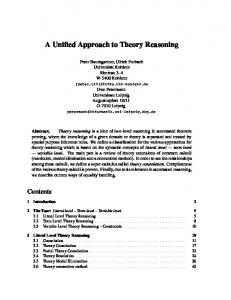
of all possible configurations of dynamic and measurement costs attainable at time T, conditional on the given observation sequence Yr. The cost-efficient frontier CF (T) is then defined to be the collection of all cost vectors c = (cg, c~) in C(T) which are not subordinated by any other cost vector c* in C(T) in the sense that c* 5 c. Formally, letting “vmin” denote vector-minimization, CF( ZJ = vmin C( 23.

(11)

By construction, then, the cost-efficient frontier is the collection of all cost vectors associated with the FLS state sequence estimates. Ifthe N x Tmatrix [hi,. . . , hT] has full rank N, the cost-efficient frontier CF( T) is a strictly convex curve in the cD-c,+, plane giving the locus of vectorminimal costs attainable at time T, conditional on the given observations. In particular, CF( ZJ reveals the measurement cost cM that must be paid in order to achieve the zero dynamic cost (time-constant state vector estimates) required by OLS estimation. [See Figure 1.1 Once the FLS estimates and the cost-efficient frontier are determined, three different levels of analysis can be used to investigate the incompatibility of the theoretical relations (7) and the observations yl, . . . , y,. First, the frontier can be examined to determine the efficient attainable trade-offs be-

LEIGH TESFATSION AND ROBERT KALABA

CD

0 (0)

Cost

Possibility

Set

C(T)

CD

0 (b)

Cost-

Efficient

Frontier

CF(T)

Fig. l(a). Cost possibility set C(T) Fig. l(b). Cost-efficient frontier C’(T)

tween the measurement and dynamic costs c,+, and CD. Second, descriptive summary statistics, e.g., average value and standard deviation, can be constructed for the time-paths traced out by the FLS estimates at each point along the frontier. These summary statistics provide rough indicators of the extent to which the FLS estimates deviate from the OLS solution associated with the extreme point of the frontier where dynamic cost is zero. Finally, the time-paths traced out by the FLS estimates can be directly examined for evidence of systematic movements in individual state variables, e.g., unanticipated jumps at dispersed points in time. These movements might be difficult to discern from summary statistical characterizations of the time-paths. A detailed theoretical discussion of the FLS technique is given in [4-61. A Fortran program for generating the FLS estimates is provided in Kalaba and Tesfatsion [5]; and simulation experiments demonstrating the ability of the FLS estimates to track linear, quadratic, sinusoidal, and regime shift motions in the true state variables, despite noisy observations, are reported and graphically depicted. In Tefatsion and Veitch [13], the FLS technique is used to undertake an empirical investigation of a well-known log-linear regression model for U.S. money demand over the volatile period 1959:Q2_1985:Q3. Interesting insights are obtained concerning shifts in the money demand relation at economically reasonable points in time. 4.

GENERALIZATIONS

In the previous section it is shown how a multicriteria approach might be used to investigate the basic incompatibility of theory and data for one type

A UNIFIED

APPROACH

TO DYNAMIC

ESTIMATION

167

of filtering and smoothing problem. This multicriteria approach is generalized in Kalaba and Tesfatsion [7] to a much broader class of problems. The present section briefly reviews this work. Consider a situation in which a sequence of observations Y7 = (y,, . . . , y7) has been obtained on a process over time periods 1, . . . , T. The basic problem is to learn about the sequence of states XT = (x, , . . , xT) through which the process has passed. Suppose the degree to which each possible state sequence estimate X7 is incompatible with the given observation sequence YT is measured by a Kdimensional vector c(X~, Y,, 7J of incompatibility costs. These costs may represent penalties imposed for failure to satisfy criteria conjectured to be true (theoretical relations), and also penalties imposed for failure to satisfy criteria preferred to be true (objectives). Let C(T) denote the set of all incompatibility cost vectors c = c(J?,. YT, T) corresponding to possible state sequence estimates X7. The cost-efficientfrontier, denoted by CF(T). is then defined to be the collection of cost vectors c in C(T) which are not subordinated by any other cost vector c* in C(T) in the sense that c* I c. By construction, the state sequence estimates XT whose cost vectors attain the cost-efftcient frontier are characterized by a basic efficiency property: for the given observations, no other possible state sequence estimate yields lower incompatibility cost with respect to each of the K modeling criteria included in the incompatibility cost vector. Each of these state sequence estimates thus represents one possible way the actual process could have evolved over time in a manner minimally incompatible with the prior theoretical relations and objectives. The basic multicriteria estimation problem can be summarized as follows:

The Basic Multicriteria

Estimation

Problem

Given a process length T, an observation sequence YT, and a multidimensional incompatibility cost function c(., Y7, T), determine all possible state sequence estimates k 7 which vector-minimize the incompatibility cost c(k,, YT, T). That is, determine all possible state sequence estimates R, whose cost vectors c(_j?,, Y7, T) attain the cost-efficient frontier CF(T). A vector-valued recurrence relation is established for the cost-efficient frontier in Kalaba and Tesfatsion [7]. This recurrence relation is readily recognizable as a multicriteria extension of the usual scalar dynamic programming equations. To give a rough idea of this result, consider the estimation problem at any intermediate time t. Suppose a K-dimension vector c(X,, Y,, t) of incompat-

168

LEIGH TESFATSION AND ROBERT KALABA

ibility costs can be associated with each t-length state sequence estimate 2, = (R,, * * . , R,), conditional on the sequence of observations Y: = (y, , . . . , y,). Let C(.f,, t) denote the set of all cost vectors c&;, Y,, r) attainable at time t, conditional on the time-t state estimate being i,; and let CF(&, t) denote the cost-efficient frontier for C(9, t). Given certain regularity conditions, it is shown that state-conditional frontiers at time t are mapped into state-conditional frontiers at time f + 1 in accordance with a vector-valued recurrence relation having the form

CF(-f,+1, t + 1) = vmin (U,,[CF(R,, t) +

WC,

%+I,

yt+l,

t + 1)lh

(12)

where “vmin” denotes vector-minimization and SC(*) denotes a vector of incremental costs associated with the state transition (a,, R,,,). Moreover, the cost-efficient frontier at the final time T satisfies f?(T)

= vmin [UmTCF(RT,Z)].

(13)

Three well-known state estimation algorithms are derived in Kalaba and Tesfatsion [7] as scalar-criterion special cases of the multicriteria recurrence relations (12) and (13): namely, the Kalman [8], Viterbi [3, 141, and LarsonPeschon [IO] filters for sequentially generating maximum a posteriori probability estimates. In addition, an algorithm for sequentially generating the FLS estimates for the problem discussed above in Section 3 is derived as a bicriteria special case of (12) and (13). 5.

CONCLUDING REMARKS

The specification of appropriate criteria for measuring the incompatibility of theory and data is a key issue for state estimation. The general multicriteria framework outlined in Section 4 provides an organizing principle for state estimation which accommodates a broad range of perspectives on this issue. If available, probability assessments can be used to provide a single scalar measure of incompatibility, as illustrated in Section 2. Alternatively, disparate sources of information can be systematically considered without forced scalarization, as illustrated in Section 3. Future studies will stress both theoretical developments and practical applications. For example, the state sequence estimates whose costs attain the cost-efficient frontier constitute a “population” of estimates characterized by a basic efficiency property: For the given observations, these are the state sequence estimates which are minimally incompatible with the prior theoretical relations and objectives. Systematic procedures need to be developed

A UNIFIED APPROACH TO DYNAMIC ESTIMATION

169

for interpreting and reporting the behavior displayed by these estimates in both simulation and empirical studies. A second related issue concerns the use of the posterior information embodied in the cost-efficient frontier for adaptive model respecification. For many years filtering and smoothing studies have primarily dealt with situations where theoretical specifications are essentially correct and model discrepancy terms are reasonably modeled as random quantities with known distributions. More recently, however, the social and biological sciences have presented filtering and smoothing problems of critical importance for which the underlying relations are not well understood. In such areas, model misspecification is an endemic problem, and procedures are needed for coping with this reality. As suggested in this paper, the explicit recognition of model specification errors raises a number of new and interesting challenges for filtering and smoothing theory. REFERENCES I. B. D. 0. Anderson and J. B. Moore, Optimal Filtering, Prentice-Hall, 1979. 2. R. Bellman and L. Zadeh, Decision-making in a fuzzy environment, Management Science 17:141-164 (1970). 3. G. D. Fomey, Jr., The Viterbi algorithm, Proceedings of the IEEE, March:268278 (1973). 4. R. Kalaba and L. Tesfatsion, Sequential nonlinear estimation with nonaugmented priors, Journal of Optimization Theory and Applications 60:421-438 (1989). 5. R. Kalaba and L. Tesfatsion, Time-varying linear regression via flexible least squares, International Journal of Computers and Mathematics with Applications 17:1215-1245 (1989). R. Kalaba and L. Tesfatsion, Flexible least squares for approximately linear systems, IEEE Transactions on Systems, Man, and Cybernetics 20: (1990). R. Kalaba and L. Tesfatsion, An organizing principle for dynamic estimation, Journal of Optimization Theory and Applications 64445-470 (1990). R. E. Kalman, A new approach to linear filtering and prediction problems, Transactions of the ASME: Journal of Basic Engineering 82:35-45 (1960). N. T. Koussoulas, Multiobjective optimization in adaptive and stochastic control, in Control and Dynamic Systems 25 (C. T. Leondes, Ed.), Academic Press, 1987, pp. 5578. 10. R. E. Larson and J. Peschon, A dynamic programming approach to trajectory estimation, IEEE Transactions on Automatic Control 11:537-540 (1966). 11. M. Salukvadze, Vector-valued Optimization Problems in Control Theory, Academic Press, 1979. 12. P. Swerling, First order error propagation in a stagewise smoothing procedure for satellite observations, Journal of the Astronautical SciencesVI:46-52 (1959). 13. L. Tesfatsion and J. Veitch, U.S. money demand instability: a flexible least squares approach, Journal of Economic Dynamics and Control 14:151-173 (1990). 14. A. J. Viterbi, Error bounds of convolutional codes and an asymptotically optimal decoding algorithm, IEEE Transactions on Information Theory 13:260-269 (1967).

Received 18 September 1989; revised 24 July 1990