AS, Research Department, Vollsveien 13C, N-1324 Lysaker, Norway.d Was at the Physics Department,. University of Oslo, now at Schlumberger Geco-Prakla, ...
1D and 2D Algorithmically Optimized Sparse Arrays Andreas Austeng a, Sverre Holm a, Peter K. Weber b, Niels Aakvaag c, and Kambiz Iranpour d Informatics, University of Oslo, P. O. Box 1080, N-0316 Oslo, Norway. b Fraunhofer Institute Biomedical Engineering, Ensheimer Strasse 48, D-66386 St. Ingbert, Germany. c Vingmed Sound AS, Research Department, Vollsveien 13C, N-1324 Lysaker, Norway. d Was at the Physics Department, University of Oslo, now at Schlumberger Geco-Prakla, Solbr˚aveien 23, N-1370 Asker, Norway. a Department of
Abstract—A new criterion, minimization of maximal weighted sidelobe, is applied together with a genetic search algorithm to the problem of element placement in a discrete linear lattice. By processing RF-data, the resulting 1D sparse arrays are compared experimentally with sparse periodic arrays and arrays found with a least square optimization criterion. The images show that algorithmically optimized layouts can be found with lateral resolution and contrast comparable to sparse periodic arrays. The approach has been extended to 2D arrays. An example is given without overlap between elements on transmit and receive. The layout is optimized for both the visible and invisible region to assure a controlled behavior when steering is applied. Advantages of this approach are that it gives flexibility in the choice of beamwidth, the potential to trade off beamwidth, maximum sidelobe level and sidelobe energy, no need for apodization, and possibility to require e.g. no overlap between receive and transmit elements.
I. I NTRODUCTION To reduce scanner cost and complexity, sparse linear phased arrays can be used. These arrays have an inter element spacing larger than d, d being the element spacing in the dense array. Sparse arrays suffer from high sidelobes compared to dense arrays. The sidelobe distribution and height depend on the element placement and possibly element weighting. Finding the positions giving the best results for a given criterion is, therefore, important. Recent work discussing sparse 1D and 2D arrays and optimal element placement have suggested different strategies based on minimizing the deviation from the full array’s response, minimizing the peak sidelobes, or minimizing the integrated sidelobe ratio (ISLR) [1] – [7]. In [8], Lockwood et. al. describes a different strategy to design sparse periodic linear arrays called the Vernier method. The beam properties of these arrays have been evaluated by processing of experimental Radio Frequency (RF) data. In this paper we propose a new criterion to use with the continuous wave (CW) response in algorithms for designing sparse arrays. The criterion is used together with a genetic search algorithm to find sparse array layouts. The layouts are compared experimentally. We show that with the new criterion, it is possible to find algorithmically optimized sparse arrays with performance compareable to arrays designed with the Vernier method. To demonstrate the flexibility of algorithmic optimization, a criterion that minimizes the difference in the radiation pattern between a sparse and dense array is also used to find layouts where This work was partly sponsored by the ESPRIT program of the European Union under contract EP 22982 and by the Norwegian Research Council (NFR) under contract 116831/320.
the beamwidth is traded off with sidelobe energy. The quality of the images constructed with the sparse layouts are compared to quantities derived from the CW response to justify the proposed criterion and the basis for the optimization algorithms. The ideas used for 1D array optimization are then extended to 2D array optimization. We show that it is possible to find algorithmically optimized steerable 2D layouts with CW response comparable to periodic 2D layouts. II. S PARSE
PERIODIC LINEAR ARRAYS
As a reference for our work, we have used sparse periodic linear arrays. This strategy, called the Vernier method by Lockwood et. al. [8], gives a simple way to design sparse linear arrays. In an attempt to maximize the signal-to-noise ratio, only nonapodized sparse arrays are considered in this paper. They will therefore be compared to rectangular apodized vernier arrays. Although this increases the secondary lobes in the radiation pattern, we feel that especially for 2D arrays, apodization should not be used due to the low element sensitivity. The rectangular apodized vernier array still gives good quality images compared to a random sparse array. III. O PTIMIZATION
CRITERIA
To demonstrate the flexibility of algorithmically optimized arrays, two different optimization criteria are used. The first one has to our knowledge not previously been applied to array optimization. The second criterion is based on the method described in [1]. A. Minimizing the maximal weighted sidelobe To be able to define a criterion for finding layouts which can compete with the performance of the vernier array, the fact that the excitation is pulsed is utilized. This is based on the following idea: The peak from a grating lobe appearing in a CW response will, when a pulsed excitation is used, be smeared out in time. The shorter the pulse and the larger the steering angle, the lower the pulsed peak response will be. Disregarding the directivity of each element, an equal amount of energy will be sent in the direction of the grating lobe as in the direction of the mainlobe, but the energy will arrive over a longer time interval. Arrays constructed with the Vernier method exploit this fact. The desired CW response is allowed to contain peaks or suppressed grating lobes at large angles. This would make it pos-
TO APPEAR IN PROC. IEEE ULTRASONIC SYMP., TORONTO, OCT. 1997
2
shown in Figure 2. Layouts A and B in Figure 2 are optimized to have a -6 dB beamwidth equal to the vernier array. This is done to simplify the comparison. Layout C has a slightly larger beamwidth. The data for the CW two-way beampatterns are summarized in the first four columns of Table I. The vernier array (Tx: 31 el.; Rx: 31 el.) 2−way response to unweighted array 0
[dB], ISLR −21.17, Avg −50.17
sible to lower the sidelobe level at smaller angles. Ideally, the elements contributing to the peak should be spaced as far from each other as possible to fully utilize the effect of pulsing. This last point is difficult to satisfy when using the CW response to evaluate the different candidates. The resulting optimization criterion is minimization of a maximal weighted sidelobe. We wanted to find responses similar to the one sketched in Figure 1. This is achieved by multiplying the response with a weight vector which equals one in the center region and decreases to zero for large angles.
Peak: −27.7 [dB]
−6 dB BW: 0.92 [deg]
−20
−40
−60
−80
dB
−20 −100 −1
−40 −60
−0.6
−0.4
−0.2
0 sin(phi)
0.2
0.4
0.6
0.8
1
Layout A (Vernier Tx, 31 el.; Optim. Rx, 31 el.) −0.8
−0.6
−0.4
−0.2
0 sin(phi)
0.2
0.4
0.6
0.8
1
Fig. 1. Sketched two-way responses of the vernier array (drawn with a solid line) and a possible desired array drawn with a dashed line.
2−way response to unweighted array,
−20
−40
−60
−80
−100 −1
B. Minimizing the error energy
Eerr
N X ∝ (Pj,dense − Pj,sparse )2 ,
Transmitter: Receiver:
· · · 00100100100100100100100 · · · · · · 00010001000100010001000 · · ·
In total, the probe has 55 connected elements (7 elements overlap between transmitter and receiver) [8][9]. To make the most out of a random or algorithmically optimized sparse array, all 55 connected elements should be considered used. In this paper, three different approaches are described. The first two are found by minimizing the maximal weighted sidelobe criterion. The first one, Layout A, uses different elements on transmitter and receiver. The transmitter pattern is chosen equal to the vernier array transmitter. The receiver pattern is optimized to achieve an optimal two-way response. The second approach, Layout B, tries to optimize all 55 elements, using the same configuration for both transmit and receive. The third approach, Layout C, uses the minimization of error energy criterion to optimize 55 elements for both transmit and receive. The layout and the CW response for the vernier array and one candidate for each of the approaches described above are
−0.2
0 sin(phi)
0.2
0.4
0.6
0.8
1
Layout B (Optim. Tx/Rx, 55 el.) −6 dB BW: 0.92 [deg]
−20
−40
−60
−80
−100 −1
−0.8
−0.6
−0.4
−0.2
0 sin(phi)
0.2
0.4
0.6
0.8
1
Thinning pattern (57.0% thinned): 1000000100100100100101010100101000101010101101011110101010110101 0101011010101010110101010101010101001010010010100100000000000101
Layout C (Optim. Tx/Rx, 55 el.) 2−way response to unweighted array,
−6 dB BW: 1.04 [deg]
0
−20
−40
−60
−80
−100 −1
The Vernier method utilizes the ability to use different elements for transmitter and receiver. The array we use as a reference has 31 elements on both transmit and receive with different spacing between active elements (0/1 – inactive/active element):
−0.4
2−way response to unweighted array,
[dB], ISLR −15.99, Avg −41.24
IV. LAYOUTS
−0.6
0
j=1
where P is the pressure at a given point. To control the beamwidth, an additional “next-neighborcriterion” was introduced. By not allowing any element to have more than two or three neighboring elements, the beamwidth was improved at the cost of a rise in peak sidelobe level.
−0.8
Thinning pattern (75.8% thinned): 1000000010000101000000000001110000010000100001000010100111000000 0011100000010000001110000001000100010100001000000000000010110001
[dB], ISLR −12.15, Avg −40.02
To construct layouts with a CW response similar to a dense array response, a second criterion based on minimization of the error energy between a dense and the sparse array is used [1]. For a given layout, the quantity minimized is
−6 dB BW: 0.92 [deg]
0
[dB], ISLR −20.52, Avg −45.28
−80 −1
−0.8
−0.8
−0.6
−0.4
−0.2
0 sin(phi)
0.2
0.4
0.6
0.8
1
Thinning pattern (57.0% thinned): 0000000000001110011100011000000000000000000000111011010110101101 1101101110110111011011101110111011101101011100011100000000000000
Fig. 2. Two-way CW response for different layouts. Layout A and Layout B are found when using the minimization of maximal weighted sidelobe criterion (see Sec. III-A). Layout C is found when using minimization of error energy criterion (see Sec. III-B).
Dense Vernier Layout A Layout B Layout C
BW 0.81◦ 0.92◦ 0.92◦ 0.92◦ 1.04◦
Peak -27 -28 -35 -43 -21
Avg -62.2 -50.2 -45.3 -40.0 -41.2
ISLR -25.3 -21.2 -20.5 -12.2 -16.0
Cexp 0.98 0.82 0.81 0.74 0.87
TABLE I CW FIGURES AND EXPERIMENTAL RESULTS. Beamwidth (BW), peak sidelobe (for sin φ ∈ [0.02-0.6]), average sidelobe and integrated sidelobe ratio is found from the CW responses. The contrast (Cexp ) is found from the cyst phantom images.
TO APPEAR IN PROC. IEEE ULTRASONIC SYMP., TORONTO, OCT. 1997
V. EXPERIMENTAL
RESULTS
The different thinning patterns were compared experimentally by processing RF data from the University of Michigan (3.5 MHz 128 el. array, pitch: 0.22 mm, sampling frequency 13.88 MHz). The images were processed using four equally spaced transmit focal zones and dynamic receive focusing as in [8]. The only difference was that we used baseband beam forming with an interpolation factor of four instead of beamforming after demodulation.
3
Point no. 1 Dense Vernier Layout A Layout B Layout C Point no. 3 Dense Vernier Layout A Layout B Layout C Point no. 6 Dense Vernier Layout A Layout B Layout C
-6db 1.00 0.97 1.01 1.14 1.24
-12dB 1.00 0.92 0.98 1.01 1.45
-24dB 1.00 0.77 0.71 0.76 0.98
-36dB 1.00 0.89 0.92 0.78 1.61
1.00 1.21 1.18 1.30 1.35
1.00 1.08 1.12 1.17 1.29
1.00 1.11 1.14 1.21 1.69
1.00 1.07 0.80 0.70 2.12
1.00 1.08 1.13 1.15 1.21
1.00 1.09 1.13 1.14 1.26
1.00 1.16 1.20 1.19 1.67
1.00 1.02 0.76 0.73 2.22
TABLE II P OINT WIDTH AT DIFFERENT LEVELS
Fig. 3. Wire target images using from top left to bottom right; the vernier array, Layout A, Layout B and Layout C. Dynamic range: 55 dB.
Figure 3 shows images of a wire phantom [10] using the layouts given in Section IV. The sidelobes in the images correlate well with the peak and average sidelobes in Table I. Layout B produces an image showing less sidelobes near broadside to the array compared to the vernier array. The image produced with Layout C shows larger near sidelobes but less energy at larger angles. The relative lateral width of the first, third and sixth point target for four different levels are tabulated in Table II. The three point targets are all close to the focal points used. All widths are normalized to the lateral width achieved with a dense array. As can be seen from the results in Table II, the vernier array and Layouts A and B have good lateral resolution ranging from about 20% above to about 30% below the results for a dense array. The sparse arrays in question were not expected to do as well as a dense array since the dense array has approximately 13% smaller -6 dB beamwidth in the CW response. Sparse arrays doing better than the dense array can partly be explained with the CW response figures, since the sparse arrays have lower first sidelobes than the dense array. If there had been a full match between the CW figures and the lateral resolution, then the lower the peak value reported in Table I, the better the expected lateral resolution. This is clearly the case for the sixth point. All arrays optimized with the new criterion have smaller peak values (see
Table I) and considerably smaller -36 dB point width than the other arrays. Layout C shows considerably poorer lateral resolution than the other layouts. This is in good agreement with the CW figures discussed in Section IV. Cyst phantom RF data [11] was then processed in order to measure contrast. The cyst phantom contains diffuse scatterers and cyst regions. The diffuse scatterers will measure the mainlobe’s ability to pick up energy, while energy appearing in the cyst region will equal the energy picked up by the sidelobe. For each layout, cyst images were constructed and the contrast estimated (see Table I). The contrast was defined as in [12]: Cexp = (S0 − S1 )/S0 , where S1 is the average level inside a region of the cyst and S0 is the average level in an equivalent region outside the cyst. The S1 and S0 values were obtained by averaging 1976 pixel values inside/outside the cyst region before any processing of the image data was performed. The S1 region was defined by placing a circle inside the area of the cyst with no observed sidelobe effect for a 60 dB dynamic range image obtained with a dense array. The S0 region is an equal-size region at the same depth in the diffuse scatter area. Table I (right-hand column) shows that Layout A and the vernier array have quite similar contrast. Layout B is doing worse and Layout C is doing better. This demonstrates the flexibility of the approach and the results correlate with the findings from the wire phantom images. The ideal case would be that the experimental contrast was correlated to the ISLR. This is not fully the case, and the mismatch is probably due to the effect of pulsing. VI. 2D
ARRAYS
The minimization of the maximal weighted sidelobe criterion can be extended to 2D arrays. We demonstrate the capability of algorithmic optimization by optimizing a typical 2D array:
TO APPEAR IN PROC. IEEE ULTRASONIC SYMP., TORONTO, OCT. 1997
4
50 × 50 elements with λ/2 pitch and frequency 2.5 MHz [13]. The array is compared to a 2D vernier array with an element spacing of λ for the transmitter (253 el.) and 1.5λ for the receiver (241 el.) and rectangular apodization. The CW figures for the periodic sparse layout are given in Table III. As for Layout A in Section IV, we choose to use the same transmitter as the vernier array, and optimize the receiver. As extra constraints for the optimized layout, we require that the transmitter should be inscribed in a circle similar to the vernier receiver, and that there should be no overlap between transmitter and receiver elements. This last constraint may be important to simplify hardware construction. Figure 4 shows the vernier transmitter and the optimized receiver layout together with three CW responses; the two-way unsteered CW response, the CW response when steering is applied and the CW response of the vernier array. The CW figures for the optimized layout are given in Table III.
The CW responses show that for the optimized layout, the peak sidelobes have decreased resulting in a larger flat area at the cost of increased average sidelobe and sidelobe energy. The increased sidelobe energy is correlated to the increased average sidelobe. Figure 4 includes the CW response when steering is applied to the sparse layout (θ = 30◦ , φ = 30◦ ). Note that the wlwmwnts are assumed to be omnidirectional. As can be seen, no extra sidelobes arise. This is due to the fact that the response has been optimized in the square region given by u, v ∈ [−1, 1] where u = sin φ cos θ and v = sin φ sin θ, rather than the circular visible region [5]. This again demonstrates the flexibility of algorithmic optimization. VII. C ONCLUSION Algorithmic optimization gives a flexible way to find sparse arrays. The approach has the possibility to trade off lateral resolution with contrast. By using minimization of the maximal weighted sidelobe, layouts with performance comparable to vernier arrays can be found. This has been verified by processing RF data from 1D arrays. The approach is extendible to 2D arrays and it is simple to include constraints like no overlap between transmit and receive elements. Performance is expected to compare well with sparse periodic 2D arrays. R EFERENCES [1] [2] [3] [4] [5] [6] [7]
−100
−80
−60
−40
−20
dB
0
Fig. 4. Layout and CW response. From top left to bottom right: 1) Layout of an optimized receiver (cross; 256 el.) and a vernier transmitter (squares; 253 el. (every second)). 2) The resulting two-way CW response. 3) The CW response when steering is applied (θ = 30◦ , φ = 30◦ ). 4) CW response for a vernier 2D array (Tx: 256 el. (every second), Rx: 241 el. (every third)). The CW responses are plotted for −1 ≤ u, v ≤ 1, u = sin φ cos θ and v = sin φ sin θ.
[8] [9] [10] [11] [12]
Optimized Periodic
BW 2.7◦ 2.6◦
a
Peak -24.9 -30.7
b
Peak2 -40.4 -33.0
Avg -58.3 -67.4
TABLE III CW FIGURES FOR 2D ARRAYS . a Peak:
u, v ∈ [−1, 1]. √ r ≤ 0.9, r = u2 + v2 .
b Peak2:
ISLR 3.3 -1.0
[13]
P. Weber, R. Schmitt, B. D. Tylkowski, and J. Steck, “Optimization of random sparse 2-D transducer arrays for 3-D electronic beam steering and focusing,” in Proc. IEEE Ultrasonics Symp., vol. 3, pp. 1503–1506, 1994. D. O’Neill, “Element placement in thinned arrays using genetic algorithms,” in Proc. OCEANS ’94, vol. 2, pp. 301–306, Sept. 1994. A. Trucco and F. Repetto, “A stochastic approach to optimizing the aperture and the number of elements of an aperiodic array,” in Proc. OCEANS ’96, vol. 3, pp. 1510–1515, Sept. 1996. V. Murino, A. Trucco, and C. S. Regazzoni, “Synthesis of unequally spaced arrays by simulated annealing,” IEEE Trans. Signal Processing, vol. 44, pp. 119–123, Jan. 1996. S. Holm, B. Elgetun, and G. Dahl, “Properties of the beampattern of weight- and layout-optimized sparse arrays,” IEEE Trans. Ultrason., Ferroelect., Freq. Contr., vol. 44, pp. 983–991, Sept. 1997. C. Boni, M. Richard, and S. Barbarossa, “Optimal configuration and weighting of nonuniform arrays according to a maximum ISLR criterion,” in IEEE Int. Conf. Acoust., Speech, Sign. Proc., vol. V, pp. 157–160, 1994. S. Holm, “Maximum sidelobe energy versus minimum peak sidelobe level for sparse array optimization,” in Proc. IEEE Nordic Signal Processing Symp., (Espoo, Finland), pp. 227–230, Sept. 1996. (Found at http://www.ifi.uio.no/˜ftp/publications/preprints/SHolm-5.ps). G. R. Lockwood, P.-C. Li, M. O’Donnell, and F. S. Foster, “Optimizing the radiation pattern of sparse periodic linear arrays,” IEEE Trans. Ultrason., Ferroelect., Freq. Contr., vol. 43, pp. 7–14, Jan. 1996. G. R. Lockwood, Jan. 1997. Personal communications. “Ultrasound RF data set acuson17 from the Univ. of Michigan.” Found at http://bul.eecs.umich.edu/. “Ultrasound rf data set cyst4 a100 from the Univ. of Michigan.” Found at http://bul.eecs.umich.edu/. D. H. Turnbull, P. K. Lum, A. T. Kerr, and F. S. Foster, “Simulation of B-scan images from two-dimensional transducer arrays: Part I - Methods and quantitative contrast measurements,” Ultrasonic Imaging, vol. 14, pp. 323–343, 1992. M. Greenstein, P. Lum, H. Yoshida, and M. S. Seyed-Bolorforosh, “A 2.5 MHz 2D array with Z-axis electrically conductive backing.,” IEEE Trans. Ultrason., Ferroelect., Freq. Contr., vol. 44, pp. 970–977, Sept. 1997.