1
Opportunistic Large Arrays Anna Scaglione and Yao-Win Hong School of Electrical and Computer Engineering, Cornell University
[email protected],
[email protected] Abstract— In this paper, we introduce a new scheme that allows transmission from a set of asynchronous transmitters to a remote destination which, otherwise, would not be capable to forward the data individually. In our scheme the small devices form an Opportunistic Large Array (OLA) by reacting to the signal sent by a special node in the network, called the leader. The problem solution provides as a byproduct a communication technique for the network itself, based on a unique physical layer design where the signals are broadcasted to the other nodes without contending for the channel.
Let E{s2m (t)} = P, then the Mean Square Estimation Error (MSE) of the signature waveforms can be written as M SE = E{kˆsm − sm k2 } =
kmax N0 kmax P = P P SN R
(3)
where SN R = P/N0 . After the training period, the receiver can adaptively update the estimations in a decision directed mode. C. Communication between leader and nodes
I. How it works? The main goal of many applications of wireless ad hoc networks is not only the mutual communication among the nodes themselves but also to enable the transmission of locally generated data to a distant receiver which has extremely low SNR with respect to each individual node. In this paper, a set of ad hoc wireless nodes are used to form an Opportunistic Large Array (OLA) by responding to the signal of the transmission leaders. In this way, the nodes in the network create an avalanche of signals similar to the ola performed by the spectators in a stadium. The OLA structure provides fast reliable transmission and diversity with very simple node cooperation. The multi-node diversity provided is in both spatial and temporal. A. The transmitter alphabet Let the leader transmit an M-ary pulse pm (t), the complex envelope of the resulting signal at the receiver is r(t) =
N X
An pm (t − τn ) + n(t) = sm (t) + n(t)
(1)
n=1
where N is the number of nodes and An is the complex fading coefficient of the nth node and sm (t) is the received mth signature signal. For a network which is sufficiently dense, the emission of multiple transmitters will be superimposed and the resulting signal sm (t) will be approximately a nonstationary Gaussian random process.
The transmission scheme of OLA can also be used to distribute information among the nodes in the network without any artificial channelization. Each node in OLA receives a multitude of signals that interfere with each other during the flooding of information, producing an effect similar to multipath. Let the signal at node i be ri (t) =
Ni X
II. OLA Modulations The OLA transmitter works with standard modulation techniques, coherent or incoherent (the structure of the OLA detectors will be omitted for brevity). A. Linear Modulation The baseband equivalent signal of the leader in this case is simply sm p(t) where sm is the complex symbol out of an M − ary constellation (QAM, ASK, PSK). Therefore,
B. The signal estimation and receiver training
N X
An p(t − τn ) = sm g(t)
(5)
n=1
At the receiver we filter the signal over the pulse bandwidth and sample r(t) at the Nyquist rate, collecting the samples in a vector r(i) = sm + n(i). The Maximum Likelihood Estimation (MLE) of sm is P 1 X r(i). P i=1
(4)
and the parameters (Ni , An,i , τn,i ) are different for all i. Hence, we apply the same training procedure as a remote receiver to estimate the signal. Therefore, all the nodes have to know the training sequence and initially react only by detecting the power variations of the incoming signal, while the pulses to sent in the training phase are an hardcoded training sequence.
sm (t) = sm
ˆsm =
An,i pm (t − τn,i ) + ni (t)
n=1
(2)
where g(t) is the transmission pulse. B. Orthogonal Signals In OLA-FSK, the mth symbol waveform is sm (t)
∼ = ej2πfm t
N X n=1
An e−j2πfm τn = gej2πfm t
(6)
where we assume that the tone duration Tp is sufficiently long. In this case, training is not strictly necessary since the signal sm (t) can be incoherently detected. In OLA-PPM the information is encoded in the time epoch of the pulse: N X
An p(t − τn − mδ) = g(t − mδ),
(7)
n=1
PN where g(t) = n=1 An p(t − τn ), and the detection can be done by a simple matched filter. The nice aspect of the OLA-PPM scheme is that it would be fully compatible with an Ultra-Wideband Radio Interface [1]. Another form of orthogonal modulation is the Leader Position Modulation. LPM is a modulation technique uniquely suitable for OLA systems. Let there be M different leaders in the network, and the mth symbol waveform is triggered by the mth leader, sm (t) =
References [1]
N X
An(m) p(t − τn(m) ).
(8)
n=1
If the positions of the leaders are sufficiently spread the (m) coefficients An are uncorrelated and the signals sm (t) are approximately independent Gaussian pseudo-noise sequences. The advantage of LPM is that all nodes transmit just one type of pulse, hence the followers only have to react to the received power variations without any decoding. Example II-B. 1: For a 4-ary LPM signal, we can locate the leaders at (3000, 0) and (0, 3000), (−3000, 0), and (0, −3000). Fig.1, shows that the correlation between different symbol waveforms is small compared to its autocorrelation. This shows that the LPM is also an orthogonal modulation.
[2]
Moe Z. Win and Robert A. Scholtz, “Ultra-Wide Bandwidth Time-Hopping Spread Spectrum Impulse Radio for Wireless Multiple-Access Communications,” IEEE Transactions on Communications, vol. 48, no. 4, April 2000. John G. Proakis, “Digital Communications (4th ed.),” McGraw Hill, New York, 2001
0 0.5
1
1.5
2
2.5
3
3.5
4
4.5 node 2
1 0.5 0 0.5
1
1.5
2
2.5
3
3.5
4
4.5 node 3
1 0.5 0 0.5
1
1.5
2
2.5
3
3.5
4
4.5
3.5
4
4.5
1 node 4 0.5 0 0.5
1
1.5
2
2.5
3
Leader Position Modulation Level
Fig. 1. Correlation between different LPM waveforms
0
10
−2
10
III. Numerical Results and Conclusions
−4
10
Probability of error
Imperfect estimation of the signal space increases the equivalent noise of the received signal. Using the union bound [2], we have s 2 ˆ dmin Pe ≤ (M − 1)Q (9) 2(N0 + max M SE)
node 1
1 0.5
Normalized Correlation
sm (t) =
techniques that exploits the positioning diversity of the ad hoc nodes. A major advantage of OLA is that reliable transmission can be achieved because of its high robustness over non-ideal environment such as fading and multipath. OLA can also be easily built on top of any existing ad hoc systems without changing their original structure.
−6
10
−8
10
−10
10
−12
10
One node transmitting P=kmax P=10kmax P=100kmax P=1000kmax
−14
In Fig.2, we show the symbol error rate (SER) for a BPSK OLA system versus the SNR of a single node. We can clearly see that it is not possible to achieve reliable transmission without the joint transmission structure of OLA. Furthermore Fig.2 we can observe that the performance can be improved by increasing the number of training symbols. However the improvement is negligible when P is larger than 10 times kmax . In conclusion, OLA is a transmission technique using the diversity nature of the random positioning of the nodes in an Ad Hoc network. A simple cooperating mechanism is introduced to exploit the joint transmission capability of distributed nodes in the network. We have shown that OLA can apply both existing or newly designed modulation
10
−16
10
−30
−25
−20
SNR for single node
Fig. 2. OLA BER versus node SNR
−15