2000: a framework for response surface methodology for simulation ...

Proceedings of the 2000 Winter Simulation Conference J. A. Joines, R. R. Barton, K. Kang, and P. A. Fishwick, eds.

A FRAMEWORK FOR RESPONSE SURFACE METHODOLOGY FOR SIMULATION OPTIMIZATION

H. Gonda Neddermeijer

Gerrit J. van Oortmarssen

Econometric Institute and Department of Public Health Erasmus University Rotterdam 3000 DR Rotterdam THE NETHERLANDS

Department of Public Health Erasmus University Rotterdam 3000 DR Rotterdam THE NETHERLANDS

Nanda Piersma Rommert Dekker Econometric Institute Erasmus University Rotterdam 3000 DR Rotterdam THE NETHERLANDS

ABSTRACT

simulation models that we consider only have real-valued parameters in the optimization, so we exclude strictly integer and qualitative parameters. RSM is a collection of statistical and mathematical techniques useful for optimizing stochastic functions (Myers and Montgomery 1995), not primarily in simulation. It is frequently used for the optimization of stochastic simulation models (Fu 1994, Carson and Maria 1997, Kleijnen 1998). This methodology is based on approximation of the stochastic objective function by a low order polynomial on a small subregion of the domain. The coefficients of the polynomial are estimated by ordinary least squares (OLS) applied to a number of observations of the stochastic objective function. To this end, the objective function is evaluated in an arrangement of points referred to as an experimental design (Kleijnen 1998). Based on the fitted polynomial, the local best point is derived, which is used as a current estimator of the optimum and as the center point of a new region of interest (Fu 1994), where again the stochastic objective function is approximated by a low order polynomial. There is a vast amount of papers and books on RSM. For extensive information on various aspects of RSM we refer to Box and Wilson (1951), Box, Hunter and Hunter (1978), Box and Draper (1987), Myers and Montgomery (1995) and Khuri and Cornell (1996). Hood and Welch (1993) give an outline of RSM when applied to non-automated optimization of simulation models. In such non-automated optimization, RSM is an interactive process in which one gradually gains understanding of the nature of the stochastic objective function. Based on these insights, the algorithm

We develop a framework for automated optimization of stochastic simulation models using Response Surface Methodology. The framework is especially intended for simulation models where the calculation of the corresponding stochastic response function is very expensive or timeconsuming. Response Surface Methodology is frequently used for the optimization of stochastic simulation models in a non-automated fashion. In scientific applications there is a clear need for a standardized algorithm based on Response Surface Methodology. In addition, an automated algorithm is less time-consuming, since there is no need to interfere in the optimization process. In our framework for automated optimization we describe the many choices that have to be made in constructing such an algorithm. 1

INTRODUCTION

When optimizing a stochastic simulation model, one tries to estimate the model parameters that optimize specific stochastic output of the simulation model. In this optimization procedure, the simulation model is often considered as a black-box model (Pflug 1996) where the output of the simulation model can be regarded as a stochastic function of the model parameters. In this paper we propose a framework for a fully automated Response Surface Methodology (RSM) for the optimization of stochastic simulation models. This framework is especially intended for simulation models where the calculation of the corresponding stochastic objective function is very expensive or time-consuming. The

129

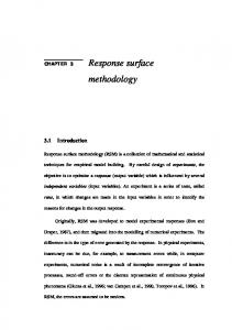
Neddermeijer, van Oortmarssen, Piersma, and Dekker simulation model. It is assumed that a screening phase, in which factors that are considered unimportant are eliminated from the optimization problem, as well as possible transformations of the factors and the response, have already taken place. Usually, a RSM algorithm comprises two phases. In the first phase the response surface function is approximated by first-order polynomials, until a polynomial is fitted that shows significant lack-of-fit, or until there is no direction of improved response anymore (Cochran and Cox 1962). In the second phase the objective function is approximated by a second-order polynomial (Fu 1994). On the basis of the various extensions and modifications of this classic algorithm that can be found in the literature, we constructed a framework for an automated RSM algorithm, see Figure 1. The various elements of this framework are described in the remainder of this paper. In each iteration n, n ≥ 1, we consider a small subregion of the domain, which is called the region of interest and is given by the k-dimensional rectangle

can be adapted during the optimization exercise. In an automated RSM algorithm, however, human intervention during the optimization process is excluded. A good automated RSM algorithm should therefore include some degree of self-correction mechanisms (Box and Liu 1999). The establishment of a clear and consistent RSM optimization algorithm is of significant importance for its use as a tool in scientific applications, e.g. , for estimation of model parameters, where results should be reproducible and derived via a clear method. A complete and clear definition of all steps and choices in a RSM algorithm is also necessary for automated optimization where all choices concerning the algorithm have to be made at the outset of an application. Automated optimization is less time-consuming, since there is no need to interfere in this optimization process. This is an advantage in large-scale time-consuming applications. However, there is no consensus about such a standard RSM algorithm. For the optimization of stochastic simulation models several methods can be used, such as RSM, the Nelder and Mead simplex method (Neddermeijer et al. 1999) and Simultaneous Perturbation Stochastic Approximation (Fu and Hill 1996). There are surprisingly few papers that systematically compare the performances of these optimization methods. Such a comparison clearly requires a standardized RSM algorithm. Smith (1976) was the first to describe an automated RSM program, without elaborating on the choices that are made within the RSM algorithm used in this program. Joshi, Sherali and Tew (1998) describe an enhanced algorithm for RSM, and compare this algorithm with a standard RSM algorithm, again without detailing this standard algorithm. In this paper we will propose a framework for a RSM algorithm for automated simulation optimization. Obviously, this framework can also be used for non-automated optimization. We will discuss the choices that have to be made when constructing a standard RSM algorithm, and we will mention references. 2



   l1n , un1 × ... × lkn , unk

This region can be described by a center point ξin =

lin + uni , i = 1, ..., k 2

and step sizes
cin = uni − lin /2, i = 1, ..., k At the start of the algorithm, an initial starting point and initial step sizes should be given. Choosing the initial step sizes at the start of the algorithm should be done with extreme caution, as we will discuss below. A. Approximate the simulation response function in the current region of interest by a first-order model. The first-order model is given by

THE FRAMEWORK y = α0 +

Without loss of generality, we assume that the optimization is a minimization problem. Mathematically, this problem can be described by

k X

αi ξi + 

i=1

We assume that the additive error  has a normal distribution with mean 0 and constant variance σ 2 . To increase the numerical accuracy in estimating the regression coefficients, the factors are coded, which gives the coded variables xi , i = 1, ..., k:

minimize f : D → IR, D ⊆ IRk where f (ξ1 , ..., ξk ) = IE (F (ξ1 , ..., ξk )); F (ξ1 , ..., ξk ) denotes the stochastic output for given input {ξ1 , ..., ξk }, and IE (F (ξ1 , ..., ξk )) denotes its expected value. When optimizing a simulation model, the arguments ξ1 , ..., ξk represent the parameters of the simulation model. In RSM, the parameters of the simulation model are usually called factors, whereas the stochastic output is called the response of the

xi =

130

ξi − ξin =⇒ ξi = cin xi + ξin cin

Neddermeijer, van Oortmarssen, Piersma, and Dekker

Start

A) Approximate the response surface function locally by a first-order model

B) Test the first-order model for adequacy C) Perform a line search in the steepest descent direction

D) Solve the inadequacy of the first-order model E) Approximate the response surface function locally by a second-order model F) Test the second-order model for adequacy

H) Perform canonical analysis

K) Determine a steepest descent direction

G) Solve the inadequacy of the second-order model

I) Perform ridge analysis

J) Accept the stationary point as the center point of the new region of interest Figure 1: Framework for an Automated RSM Algorithm

131

Neddermeijer, van Oortmarssen, Piersma, and Dekker is used for determining the direction where improvement of the simulation response is expected. The steepest descent direction is given by (−b1 , ..., −bk ). A line search is performed from the center point of the current region of interest in this direction to find a point of improved response. This point is taken as the estimator of the optimum of the simulation response function in the nth iteration, and is used as the center point o of interest in the n of the region (n + 1)th iteration, i.e. ξ1n+1 , ..., ξkn+1 . In most RSM literature, line search is applied as follows (Box and Draper 1987, Myers and Montgomery 1995, Khuri and Cornell 1996). First, increments (11 , ..., 1k ) along the steepest descent direction are chosen, where 11 ÷...÷1k = b1 ÷ ... ÷ bk . These increments are usually determined by subjectively choosing a most important factor, e.g. , ξj . Alternatively, one could objectively choose a most important factor by determining j such that j = arg maxi=1,...,k |bi |. In both cases, the increments are set to

and the coded first-order model: Y = β0 +

k X

βi xi + 

i=1

Estimators of the regression coefficients {β0 , β1 , ..., βk } are determined by using OLS and are denoted by {b0 , b1 , ..., bk }. To this end, the objective function is evaluated in the points of an experimental design, which is a specific arrangement of points in the current region of interest. Although there are many designs to choose from, usually a fractional two-level factorial design of resolution-III (Kleijnen 1998) is used, often augmented by the center point of the current region of interest (Myers and Montgomery 1995). This design is orthogonal, which means that the variance of the predicted response in the region of interest is minimal, and that the regression coefficients can be assessed independently (Khuri and Cornell 1996). Moreover, resolution-III designs give unbiased estimators of the regression coefficients of a firstorder polynomial (Kleijnen 1998), and are practical since the number of design points is small compared to other types of two-level factorial designs. Another advantage is that this type of design can quite easily be augmented to derive a second-order design. If the design is not within the domain D, then it is moved into this region (Smith 1976). B. Test the first-order model for adequacy. Before using the first-order model to move into a direction of improved response, it should be tested if the estimated firstorder model adequately describes the behaviour of the response in the current region of interest. If the true response shows interaction between the factors or pure curvature, the estimated first-order model will likely show lack-offit, which can be assessed from the analysis of variance (ANOVA) table. Testing for lack of fit requires that the resolution-III design used for estimating the regression coefficients of the first-order model is not saturated, i.e. the total number of observations should be larger than the number of regression coefficients. Moreover, multiple observations are needed in the center point of the region of interest (Box and Draper 1987). Alternatively, one could apply crossvalidation (Kleijnen 1998). Furthermore, it could happen that although the first-order model does fit well, it is not possible to determine a significant direction of improved response from this model. This occurs when the estimated regression coefficients are not significantly different from zero, which can also be assessed using the ANOVA table. At the start of the algorithm it should be decided which of these tests to use, i.e. when to accept the first-order model. For example, if there is interaction between the factors but no pure curvature, one could still decide to accept the first-order model. The decisions include choosing the significance levels for the tests involved. C. Perform a line search in the steepest descent direction. If the first-order model is accepted, then this model

1i =

−bi , i = 1, ..., k |bj |

units in the coded variables. Another option is to set the increments (11 , ..., 1k ) equal to the distance from the center point to the point of intersection ofPthe direction of steepest descent and the sphere given by ki=1 12i = 1. (Neddermeijer et al. 1999). The mth line  search point is given by ξ1n + m11 c1n , ..., ξkn + m1k ckn . It follows that the initial step sizes chosen at the start of the algorithm have a direct effect on the magnitude of the movement of the factors, whereas it has no effect on the direction of steepest descent (Myers and Montgomery 1995). As soon as a boundary of the domain D is crossed, the line search is continued along the projection of the search direction on this boundary (Smith 1976). To end this type of line search, a stopping rule has to be chosen. The usual recommendation is to stop the line search when no further improvement is observed (Del Castillo 1997). The most straightforward rule ends the line search when an observed value of the simulation response function is higher than the preceding observation, i.e. set ξin+1 equal to line search point m if line search point m + 1 is the first line search point for which no improvement was found. This rule, however, is sensitive to the noise of the response surface function, so the new center point is probably not optimal. Therefore, Del Castillo (1997) compares this stopping rule with a number of rules that do take the noise into account. These rules include the 2-in-a-row and the 3-in-a-row stopping rules, which end the line search when 2 or 3 consecutive observed values of the simulation response function are higher than the preceding observation. In the Myers and Khuri stopping rule, however, the line search ends when an observed value of the simulation response function is significantly higher than the preceding

132

Neddermeijer, van Oortmarssen, Piersma, and Dekker (CCD) (Myers and Montgomery 1995). This design can be easily constructed by augmenting the fractional factorial design that was used for estimating the first-order model. It is common to construct the CCD in such a way that it is rotatable, which means that the variance of the predicted response remains constant at all points which are equidistant to the center point of the current region of interest (Khuri and Cornell 1996). Furthermore, the CCD can be transformed such that it is orthogonal by choosing a specific number of replicated observations in the center point of the current region of interest (Khuri and Cornell 1996, p.123). If the design is not within the domain D, then it is moved into this region (Smith 1976). F. Testing the second-order model for adequacy. Similar to the first-order model, it should be tested if the estimated second-order model adequately describes the behaviour of the response in the current region of interest before using this model. G. Solve the inadequacy of the second-order model. If the second-order model is found not to be adequate, then one can reduce the size of the region of interest (Joshi, Sherali and Tew 1998) or increase the simulation size used in evaluating a design point. In RSM it is not customary to fit a higher than second-order polynomial (Kleijnen 1998). H. Perform canonical analysis. If the second-order model is found to be adequate, then canonical analysis is performed to determine the location and the nature of the stationary point of the second-order model. The estimated second-order approximation can be written as follows:

observation. Del Castillo proposes a stopping rule with variable increments that is based on recursive estimation of second-order polynomials along the search direction. Based on simulated line searches, Del Castillo finds that both this recursive procedure and the Myers and Khuri rule perform better than the n-in-a-row stopping rules. Fu (1994) describes another type of line search algorithms where a set of experiments along the steepest descent direction is performed. From these experiments, a one-dimensional second-order polynomial is estimated. This polynomial is optimized to derive the next center point ξin+1 . Safizadeh and Signorile (1994) mention a similar line search algorithm. In addition, Joshi, Sherali and Tew (1998) introduce a line search algorithm which applies gradient deflection methods to prevent zigzagging of the steepest descent directions in multiple iterations. D. Solve the inadequacy of the first-order model. If the first-order model is not accepted, then either there is some evidence of pure curvature or interaction between the factors in the current region of interest, or the steepest descent direction cannot be discerned from zero. Usually, this is solved by approximating the simulation response function in the region of interest by a second-order polynomial. However, the optimization algorithm becomes less efficient especially if this occurs very early during the optimization exercise. Therefore, an alternative solution is to reduce the size of the region of interest by decreasing the step sizes cin , i = 1, ..., k. In this way this region can possibly become small enough to ensure that a first-order approximation is an adequate local representation of the simulation response function. Another solution is to increase the simulation size used to evaluate a design point or to increase the number of replicated observations done in the design points. This may ensure that indeed a significant direction of steepest descent is found. At the start of the algorithm it should be decided which actions will be taken when the first-order model is rejected. Different actions can be taken depending on the outcome of the tests and the stage of the optimization exercise. For example, depending on the p-value found for the lack-of-fit test, one could decide to apply a second-order approximation or to decrease the size of the region of interest. E. Approximate the objective function in the current region of interest by a second-order model. The coded second-order model is given by: Y = β0 +

k X i=1

βi xi +

k k X X

Yˆ = β0 + x0 b + x0 Bx where b

B

(b1 , ..., bk )  b1,2 /2 b1,1  b 2,2  =  

=

··· ··· .. .

sym.

b1,k /2 b2,k /2 .. .

    

bk,k

The stationary point s of the second-order polynomial is determined by 1 s = − B−1 b 2 Let E be the matrix of normalized eigenvectors of B and let v1 , ..., vk be the eigenvalues of B. If all eigenvalues are positive (negative), then the quadratic surface has a minimum (maximum) at the stationary point s. If the eigenvalues have mixed signs, then the stationary point s is a saddle point. I. Perform ridge analysis. It is not advisable to extrapolate the second-order polynomial beyond the current region of interest (Myers and Montgomery 1995). There-

βi,j xi xj + 

i=1 j =i

The regression coefficients of the second-order model are again determined by using OLS applied to observations performed in an experimental design. The most popular class of second-order designs is the central composite design

133

Neddermeijer, van Oortmarssen, Piersma, and Dekker to determine a direction of steepest descent. Next, they perform a line search using this direction, resulting in a new center of a region of interest. In this region the simulation response surface will be approximated by a first-order model. Stopping criterion. In the RSM literature, it is often proposed to end the algorithm after fitting only one second order polynomial (Fu 1994, Kleijnen 1998). However, we do not recommend this strategy for two reasons. First of all, this strategy assumes that a minimum inside the current region is found, and therefore excludes the cases in which either a minimum outside the current region is found or a maximum or a saddle point is found. Furthermore, Greenwood, Rees and Siochi (1998) find that even for simple simulation response surfaces, first-order models can be inappropriate over a large area of the domain. Depending on the choices made in the algorithm, this means that the optimization can turn to the second-order phase quite early in the optimization exercise. Consequently, if the optimization algorithm ends after only one second-order approximation, it is likely that the best point of the optimization is located far from the optimum. Therefore, we recommend ending the optimization exercise if (i) the estimated optimal simulation response value does not improve sufficiently anymore, if (ii) the region of interest becomes too small, or, in case there are budget constraints, if (iii) a fixed maximum number of evaluations have been performed. Next, a confidence interval about the response at the estimator for the optimum and the location of this estimator can be determined, see e.g. , Carter et al. (1984). We want to underline the fact that the Nelder and Mead simplex method is a local search method. No guarantee is given for finding the global optimum. Therefore, when optimizing a stochastic objective function, multistart using multiple starting points and / or multiple searches from the same starting point should be considered.

fore, if the stationary point is a minimum which lies outside the current region of interest, the stationary point is not accepted as the center of the next region of interest. If the stationary point is a maximum or a saddle point, then the stationary point is rejected as well. In these cases, ridge analysis is performed, which means a search for a new stationary point sR on a given radius R such that the second order model has a minimum at this stationary point (Myers and Montgomery 1995). Using Lagrange analysis with multiplier µ, this stationary point is given by 1 (B − µI) sR = − b 2 q 0 s = R should hold. We can and µ < mini vi and sR R write 2 k  X ei0 b 0 sR = R 2 = sR 2 (vi − µ) i=1

where ei is the eigenvector corresponding to the ith eigenvalue vi . A choice for the radius R has to be made. For example, one could consider the radius of √ the circumscribed sphere of the region of interest (R = 2), which means that we have to find µ < mini vi such that k  X i=1

ei0 b 2 (vi − µ)

2 =2

Standard numerical methods for finding the root of an equation can be used to determine µ. J. Accept the stationary point. The stationary point will be used as the center point of the next region of interest. It should be decided whether a first-order or a second-order model is used to approximate the simulation response surface in this region. These decisions can be made dependent on the results of the canonical analysis. For example, if a minimum was found, it could be useful to explore a region around this minimum with a new secondorder approximation. On the other hand, if a maximum or a saddle point was found, the optimum could still be located far away from the current region of interest. In this case, approximating this region with a first-order model and consequently performing a line search would be preferable. Allowing this return to the first phase of the RSM algorithm is a powerful self-correction mechanism (Neddermeijer et al. 1999). K. Determine a steepest descent direction from the second-order model. Joshi, Sherali and Tew (1998) introduced an enhanced RSM algorithm, in which they use the gradient of the second-order model in the center point of the current region and the results of the canonical analysis

3

CONCLUSION AND FUTURE WORK

In this paper we proposed a framework for the optimization of simulation models using Response Surface Methodology. In the RSM literature, this methodology is usually applied in a non-automated fashion, and much work is done on improving separate parts of RSM. This paper is the first attempt to define a clear, detailed and consistent RSM algorithm. The framework is especially useful for automated optimization, in which all the settings of the algorithm have to be chosen at the outset of the optimization process. Based on this framework, additional research can be done on comparing the different settings of the RSM algorithm for automated optimization of simulation models. We will show the results of this research during the 2000 Winter Simulation Conference. Furthermore, the question remains

134

Neddermeijer, van Oortmarssen, Piersma, and Dekker how the RSM algorithm compares to other algorithms such as the Nelder and Mead simplex method and Simultaneous Perturbation Stochastic Approximation.

Khuri, A. I. and J. A. Cornell. 1996. Response surfaces: designs and analyses. New York: Marcel Dekker, Inc. Kleijnen, J. P. C., 1998. Experimental design for sensitivity analysis, optimization, and validation of simulation models. In Handbook of simulation: principles, methodology, advances, applications and practice, ed. J. Banks, 173–223. New York: John Wiley & Sons. Myers, R. H. and D. C. Montgomery. 1995. Response surface methodology: process and product optimization using designed experiments. New York: John Wiley & Sons. Neddermeijer, H. G., N. Piersma, G. J. van Oortmarssen, J. D. F. Habbema and R. Dekker. 1999. Comparison of response surface methodology and the Nelder and Mead simplex method for optimization in microsimulation models. Econometric Institute Report EI-9924/A, Erasmus University Rotterdam, The Netherlands. Pflug, G. Ch. 1996. Optimization of stochastic models: the interface between simulation and optimization. Boston: Kluwer Academic Publishers. Safizadeh, M. H. and R. Signorile. 1994. Optimization of simulation via quasi-Newton methods. ORSA Journal on Computing 6(4): 398–408. Smith, D. E. 1976. Automatic optimum-seeking program for digital simulation. Simulation 27:270–31.

REFERENCES Box, G. E. P, and N. R. Draper. 1987. Empirical modelbuilding and response surfaces. New York: John Wiley & Sons. Box, G. E. P., W. G. Hunter and J. S. Hunter. 1978. Statistics for experimenters: An introduction to design, data analysis, and model building. New York: John Wiley & Sons. Box, G. E. P. and P. Y. T. Liu. 1999. Statistics as a catalyst to learning by scientific method part I - an example. Journal of Quality Technology 31(1): 1–15. Box, G. E. P. and K. B. Wilson. 1951. On the experimental attainment of optimum conditions. Journal of the Royal Statistical Society, Series B 13(1): 1–38. Carson, Y. and A. Maria. 1997. Simulation optimization: methods and applications. In Proceedings of the 1997 Winter Simulation Conference, eds. S. Andradóttir, K.J. Healy, D.H. Withers and B.L. Nelson, 118–126. Piscataway, New Jersey: IEEE Press. Carter, W. H., V. M. Chinchilli, E. D. Campbell and G. L. Wampler. 1984. Confidence intervals about the response at the stationary point of a response surface, with an application to preclinical cancer therapy. Biometrics 40:1125–1130. Cochran, W. G. and G. M. Cox. 1962. Experimental designs. New York: John Wiley & Sons. Del Castillo, E. 1997. Stopping rules for steepest ascent in experimental optimization. Communications in Statistics. Simulation and Computation 26 (4): 1599–1615. Fu, M.C. 1994. Optimization via simulation: a review. Annals of Operations Research 53:199–247. Fu, M.C. and S.D. Hill. 1996. Optimization of discrete event systems via simultaneous perturbation stochastic approximation. IIE Transactions 29:233–243. Greenwood, A.G., L.P. Rees and F.C. Siochi. 1998. An investigation of the behavior of simulation response surfaces. European Journal of Operational Research 110:282–313. Hood, S. J. and P. D. Welch. 1993. Response surface methodology and its application in simulation. In Proceedings of the 1993 Winter Simulation Conference, eds. G. W. Evans, M. Mollaghasemi, E. C. Russell and W. E. Biles, 115–122. Piscataway, New Jersey: IEEE Press. Joshi, S., H. D. Sherali and J. D. Tew. 1998. An enhanced response surface methodology (RSM) algorithm using gradient deflection and second-order search strategies. Computers and Operations Research 25 (7/8): 531– 541.

AUTHOR BIOGRAPHIES H. GONDA NEDDERMEIJER is a Ph.D. student at the Econometric Institute and the Department of Public Health at the Erasmus University Rotterdam, The Netherlands. She received a M.Sc. degree in technical mathematics at the Delft University of Technology, and a M.Sc. degree in Health Services Research at the Erasmus University Rotterdam. She is a member of INFORMS. Her research interests include optimization of stochastic simulation models and simulation models for screening for early detection of cancer. Her email and web addresses are and . GERRIT J. VAN OORTMARSSEN is assistant professor of Public Health at the Department of Public Health of the Erasmus University Rotterdam. He obtained his Ph.D. at the Erasmus University, and his M.Sc. degree in applied mathematics from the Twente University of Technology. His research interest is (simulation) modeling of public health interventions for diseases, in particular applied to screening for early detection of cancer, and control of tropical infectious diseases (onchocerciasis, schistosomiasis, lymphatic filariasis, leprosy, STDs). His email address is .

135

Neddermeijer, van Oortmarssen, Piersma, and Dekker NANDA PIERSMA is assistant professor in operations research at the Econometric Institute of the Erasmus University Rotterdam. She obtained her Ph.D. in operations research and her M.Sc. degree in mathematics at the University of Amsterdam. Her research interest is stochastic modeling in operations research and marketing econometrics. Her email and web addresses are and . ROMMERT DEKKER is a full professor in operations research at the Econometric Institute of the Erasmus University Rotterdam. He obtained his Ph.D. in operations research at the State University of Leiden, and his M.Sc. degree in industrial engineering from the Twente University of Technology. He worked during seven years with Shell. His current research interests are: maintenance and logistics (inventory control, spare parts, containers and reverse logistics). He has often applied simulation models in various logistical activities. His email and web addresses are and .

136