Proceedings of the 2001 Winter Simulation Conference B. A. Peters, J. S. Smith, D. J. Medeiros, and M. W. Rohrer, eds.
PREDICTION OF PROCESS PARAMETERS FOR INTELLIGENT CONTROL OF FREEZING TUNNELS USING SIMULATION Sreeram Ramakrishnan Richard A. Wysk Vittaldas V. Prabhu Department of Industrial and Manufacturing Engineering Pennsylvania State University University Park, PA 16802, U.S.A.
model incorporating temperature-dependent thermal properties is considered to be more realistic than the second approach. Most methods used to estimate dwell time requirements assume that the heat transfer in the freezing process occurs primarily due to conduction and convection. Though in practice, heat transfer at the surface of the product can occur by a combination of all or some of conduction, convection, radiation, and evaporation. The most common approach is to model the heat transfer using Newton’s law of cooling at the surface and to define an “effective heat transfer coefficient” to account for the net effect of all the actual heat transfer mechanisms involved. The difficulties in modeling the heat transfer process for irregular shaped objects necessitate the incorporation of several assumptions in the methods used to estimate freezing time. These assumptions include the existence of a steady state, uniform properties and / or shape approximations such as the object being treated as an infinite cylinder, sphere, or as a set of infinite parallel plates. The issues to be considered while selecting a freezing time estimation method, various analytical, approximate numerical and empirical methods used, the assumptions associated with each of the methods, and their fields of applications have been discussed extensively in existing literature (ASHRAE 1981, Hung and Thomson 1983, Cleland and Earle 1984, Pham 1985, Salvadori and Macheroni 1991, Hossain, Cleland and Cleland 1992). A review of existing freezing time techniques has been provided in Wysk, Prabhu, and Ramakrishnan (2000). Traditionally, the operating parameters of a freezing tunnel are maintained at levels appropriate to freeze the maximum expected thermal load, resulting in over-freezing of some of the products. Since, the maximum thermal load cannot be predicted accurately for a process involving ‘random’ input, such as that in meat processing, there exists a possibility of ‘under-freezing’ some of the products. This approach results in the wastage of refrigerant and/or
ABSTRACT Various analytical and empirical methods assuming the existence of steady state and requiring homogenous properties of the product have been used with limited success in estimating freezing times in the food processing industry. Irrespective of the method adopted for estimating freezing time requirements, a critical process issue that needs to be considered is that of system control. Simulation models suggest that a feed-forward control strategy, as discussed in this paper, can be used to control a freezing tunnel and obtain considerable energy savings while ensuring ‘appropriate’ freezing of all products. The control strategy discussed in this paper, involves the continuous monitoring of product input and controlling either or both of the refrigerant flow and conveyor speed. The primary objective of this paper is to demonstrate the use of simulation to predict process parameters for ‘intelligent control’ of freezing tunnels, and provide an estimate of potential energy savings. 1
INTRODUCTION
The estimation of freezing time requirements is critical in the operation and control of cryogenic systems. Different thermodynamic models have been developed to describe the freezing process and provide methods to estimate the “dwell time” requirements for a product to be frozen. The two main thermodynamic models are the ‘heat conduction with temperature-dependent thermal properties model’ and the ‘unique phase-change front model’ (Valentas, Rotstein, and Singh 1997). The latter model is based on the assumption that all the latent heat is released at a unique temperature at a sharp phase-change front. This front moves from the outside to the thermal center of the object being frozen. The model further assumes that the thermal properties in the regions before and after the front are constant but different. Due to the above-mentioned assumptions, the
888
Ramakrishnan, Wysk, and Prabhu model can be obtained to improve the control strategy selection process.
under-freezing of some of the products. A similar problem does not exist for operations such bottling, since the thermal load is deterministic (Wysk, Prabhu and Ramakrishnan 2000). 2
3
PROBLEM STATEMENT AND RESEARCH OBJECTIVE
SYSTEM OVERVIEW
A schematic representation of the tunnel freezing operation viewed as a single process is shown in Figure 1. The entire process can be considered to be made up of three distinct ‘components’: the conveyor system providing the input to the freezer (the products that need to be frozen), the freezing tunnel, and the conveyor system to transport the frozen products to packaging and/or storage or the next process. The process is considered to be “in control”, if no stacking of the food product is noticed in any of the conveyor segments. The treatment of the freezing process as a stochastic process and the assumptions made in the creating the simulation model has been discussed in this section.
Cryogenic freezing tunnels can be operated in a variety of modes. Typically, the industry practice is to employ a “bang-bang” control system where the cryogen flow in the system is increased or decreased based on some predefined threshold temperature values in a pre-defined location on the tunnel. Instances where the control system regulates the cryogen flow based on the temperature monitored at only one location in a multi-zone tunnel have been seen. Such control systems either result in under-freezing of the product, necessitating their “re-working” and hence an increased cycle time, or in the wastage of cryogen and a reduction in quality due to over-freezing of the products. A evaluation of alternative control strategies is therefore necessary. An ‘intelligent process control’ strategy involves the continuous monitoring of product input and the controlling of either or both of the two primary control parameters conveyor speed in the tunnel and the refrigerant flow. For each of the control options, issues such as system’s responsiveness, the time taken by the atmosphere in the tunnel to return to steady state after and the potential energy and cost savings need to be studied. A key decision in implementing ‘intelligent process control’ is the selection of the controlled parameter and the range of control. It is necessary to obtain a preliminary understanding of the system’s behavior under static control before performing a detailed analysis. Static control refers to the scenario where the operational parameters are not altered for a particular ‘run’ despite the presence of any thermal load variations. Computer simulation provides an efficient and effective way to achieve the required preliminary information. The use of simulation to provide an estimate of the energy savings in the tunnel freezing process using ‘intelligent control’ and help identify potential control strategies has been discussed in this paper. Different scenarios each involving different intelligently controlled variable(s) identified earlier, were considered. In this simulation model, the stochastic nature of the process (discussed in later sections) was represented using only two random numbers the thermal mass of the object and the inter-arrival rate. The effect of the variation in thermal mass on the performance of the freezing tunnel was also analyzed. This analysis will enable to identify a potential methodology to estimate the operational parameters for effectively controlling the tunnel-freezing process and estimate the potential savings of using ‘intelligent control’. Information from this analysis can be used to determine how a more ‘detailed’
Cryogen Feed
Storage
Product Input
Figure 1: Tunnel Freezing Process 3.1 Stochastic Elements in a Typical Tunnel Freezing Process The stochastic nature of the freezing process can be seen in the nature of product input, product to be frozen, and the issues related to production. The main issues that are related to the product input are the size and shape of the product to be frozen, the distribution of the mass, incoming temperature, and the chemical composition of the product. Depending on the portion of the product (for example chicken pieces – whole chicken, thigh, breast, etc.) being frozen, the variation seen in the mass of the individual pieces could be significant. The approximation of the shape of the product being frozen is a key factor for estimating freezing times. The thermal mass of the products (mass of each piece * specific heat capacity * change in temperature) determines if any of the controllable operating variables need to be changed when the product enters the freezing tunnel. In order to obtain a good estimate on the variations in thermal loads of the freezer, it is necessary to characterize each of the three constituent random variables that constitute the thermal mass – mass, incoming temperature, and the chemical composition of the product. Any variation in the incoming temperature of the products also needs to be captured. Even though, the sensible heat may not account for a significant portion of the heat to be removed compared to the latent heat of water removed while freezing, the effect of varying incoming temperature needs to be
889
Ramakrishnan, Wysk, and Prabhu accounts for both the sensible heat as well as the latent heat of fusion for the water content in the food object. ‘Product entities’ in the simulation model have their ‘thermal mass’ generated from a single random stream. In practice, this could be considered that all the food objects represented by the entities in the simulation model belong to one batch, i.e., chicken pieces only, beef patties only, etc. The variation among the individual pieces in each of the batches is ‘accounted’ for in the random stream. In this model, the thermal loads were assumed to be normally distributed. The mean and the standard deviation of the normal distributions were two of the variables used in the experimental design for the simulation, discussed in a later section. The two random variables considered in this initial model are the thermal mass of the food object, discussed above, and the Time Between Arrival (TBA) of the pieces. In the initial model, the TBA was assumed to be constant. This assumption is based on the observation that very often the input to the freezer is provided by an upstream “steam cooker” or a “pattie maker” which typically provides a constant stream of output. The thermal properties of the object have not been explicitly considered since the only variable associated with the individual pieces is its thermal mass. The model assumes that conditions necessary for steady state heat transfer exist in the tunnel. The freezing time requirement is estimated based on the ‘thermal mass’ for each individual piece, assuming constant conditions in the freezing tunnel. Moreover, the model assumes that the effect of any heat exchange between the tunnel’s refrigerant system and its ambience is negligible. One of the main advantages of using simulation models in this context is its inherent flexibility to incorporate and test different dwell-time estimating techniques and its subsequent use as a tool for process control. The freezing time requirement for each entity is estimated by the simulation model using the Plank’s equation. Plank developed an equation, based on the unique phase change model, for estimating freezing time for different geometrical shapes, and allowing for varying film coefficients. The equation, derived for one-dimensional infinite slab geometry has been analytically extended for infinite cylinders, spheres and for finite parallelopiped geometries. Plank’s equation as used in the model can be expressed as follows:
considered while designing an automatic control system for the freezing process. It is also necessary to know the products’ chemical composition - volume or mass fraction of water content, fat, protein, carbohydrates, fiber, and ash, to estimate the thermal properties of the pieces. Other stochastic elements in a freezing process include factors related to the process such as the spacing between products while entering the freezer and the freezing tunnel characteristics, both of which need to be considered while devising control strategies. The freezer (cryogenic) capacity of the tunnel, the temperature setting in each of the tunnel zones, and the length of each zone needs to be known. Based on this information, the number of individual pieces that will be in the freezing tunnel at any given point of time can be estimated. This is required to keep track of the ‘most constraining’ product (the one with the maximum thermal mass among the ‘entities’ currently inside the freezer) and determine when the conveyor speed needs to be changed. Factors such as the type of packaging used, the presence of air in packages, the number of packages introduced to the tunnel simultaneously (similar to the number of boards in a panel in printed circuit board assembly) also need to be considered. 3.2 Modeling Heat Transfer and Estimating Freezing Time Since the freezing front moves towards the thermal center of the object and because of the temperature-dependent thermal properties, the mathematical modeling of the freezing process for irregular-shaped objects is difficult. The two main approaches for modeling heat transfer in freezing were mentioned at the outset. In practice, however, the freezing of a food object would involve a combination of all or some of the heat transfer modes such as conduction, convection, radiation, and evaporation. The most common modeling approach is to use Newton’s law of cooling at the surface and to define an effective heat transfer coefficient to account for the net effect of all the actual mechanisms. 3.3 Assumptions in System Modeling and Simulation Analysis This section outlines the assumptions made in the design of the simulation model and their implications in the analysis. The initial finite difference freezing model created within the computer simulation does not treat the individual components (identified earlier) that make up the thermal mass separately. Since the sums and products of random variables are random variables, the thermal mass of a food object – product of the mass, specific thermal capacity and the temperature range it is subjected to, is estimated by a single thermal mass random variable. It is also assumed that the thermal mass represented by the random number
t = f θ
R R2 + − θ h 2k if a f ρL
Where: tf is the time required for freezing, R is the characteristic half thickness of the food object
890
Ramakrishnan, Wysk, and Prabhu In order to achieve process control of the tunnel freezing process, any of the following three methods can be adopted – (i) Vary the conveyor speed (keeping the operating tonnage constant) so as to accommodate the dwell time requirement of the most constraining entity in the tunnel at any given point of time (ii) Vary the refrigeration rate (keeping the conveyor speed at a set value) depending on the thermal load on the freezer at any given point of time and (iii) Vary the refrigeration rate and the conveyor speed simultaneously.
h, kf are heat transfer coefficient and thermal conductivity (before freezing) respectively θif , θa denote the freezing point and ambient temperatures. The initial model treats the entire freezing tunnel as a single segment of uniform temperature. This would correspond to the cryogen being fed into the tunnel through different locations in the tunnel so as to maintain a uniform temperature, rather than only from an end of the tunnel. In a modified version of the model, the tunnel was modeled as one with four zones with preset temperatures with the heat transfer being a combination of conduction and forced convection. Issues such as the impact of the heat generated by the fans in the tunnel, positioning of the freezer spray, the location and number of fans has not been considered at this stage. However, the control strategy discussed in this paper is independent of the method used for estimating the dwell time requirements and the treatment of the tunnel – in terms of the number of zones and temperature distribution within each zone. In a conservative control strategy, assuming normally distributed thermal loads, (thermal mass ~ Normal(µ, σ)), the thermal load corresponding to µ + 4σ will be typically used to set the conveyor speed. This speed would correspond to the lowest required conveyor speed, or the maximum required dwell time for an individual piece. It is to be noted that this setting would allow for the system to freeze atleast 99.99% of the pieces. However, a significant number of the pierces will be over-frozen. It is also likely that a small number of the pieces (less than 0.001%), whose thermal mass is greater than µ + 4σ will not be adequately frozen. Thus, in a conservative approach to control the tunnel freezing process, it is assumed that the critical design parameter is the thermal load corresponding to µ + 4σ and that the operating tonnage is fixed. Moreover, the conveyor speed in the tunnel is fixed, and corresponds to the highest required dwell time defined by the thermal mass, µ + 4σ. For the different scenarios considered in the simulation, the ‘optimum’ operating tonnage observed for each trial will be compared to the tonnage corresponding to µ + 4σ of that trial (conservative approach). An initial simulation run where the operating parameters were fixed according to the conservative approach yielded 0.0009% of products that were not frozen, as can be expected from the properties of the Normal distribution. Even though, the percentage of unfrozen ‘products’ may be negligible in most cases, the emphasis is on the overfreezing of a significant portion of the ‘products’ – more energy than required was spent on freezing most of the products since the operational parameters were set for the maximum anticipated thermal load. This inefficient usage of energy will be reduced by adopting the proposed control strategy.
4
ESTIMATION OF CONTROL PARAMETERS USING SIMULATION
Estimates on the cost and energy savings using an ‘intelligent control’ approach and the ‘optimum’ values for the operational parameters for the tunnel can be obtained using simulation models, keeping in mind the underlying assumptions in heat transfer and freezing time estimation models used in the simulation model. Moreover, the simulation model will help to obtain a preliminary understanding of the effect of variation of the thermal mass (modeled as a single random number) for a fixed mean thermal mass on the performance of the freezing tunnel. An experimental design can be used to find the lowest operating capacity required for the freezing tunnel so as to maintain the required throughput, ensuring that the process is always ‘in-control’. 5
ANALYSIS USING SIMULATION MODELS
In general, the strategy used for intelligent process control assumes that the operating tonnage of the freezer and / or the conveyor speed is ‘intelligently’ controlled depending on the most constraining entity’s (currently in the tunnel) dwell time requirement. In the first phase the performance of the system under ‘intelligent control’ where the conveyor speed was ‘adaptively’ changed in accordance with the dwell time requirement, while keeping the operating tonnage of the freezer constant, was studied. The objective was to identify the lowest feasible operating tonnage, which can be used along with ‘intelligent control’ of the conveyor speed to provide an “in-control” process. In the second phase, the simulation model was used to compare the system’s performance when the freezer capacity is used as the intelligently controlled variable. Theoretically, the total energy consumption in the two phases should be equivalent, assuming that there are no time delays involved in attaining the required temperatures whenever the refrigerant flow is altered. In the third phase, the capacity of the tunnel was initially fixed at a level corresponding to the ‘optimal’ tonnage level observed in the first phase. However, the system had the flexibility to change the conveyor speed and the capacity depending on the dwell time requirements of the entity entering the tunnel, the instantane-
891
Ramakrishnan, Wysk, and Prabhu der list’ - a list is maintained in a way such that the entities are sorted in the descending order of the required dwell time. Each time an entity exits the tunnel, its copy from the list is also deleted. The required statistics are collected and the entity is ‘disposed’ after it travels a short section after the freezer. The model input is in the form random stream for the thermal mass to be assigned to each of the entities. The operating capacity of the tunnel (in Tons) and the TBA are the other design parameters. The model collects statistics, which includes the throughput (to ensure that the process is “in-control”) to analyze the system’s performance, and the time spent by each entity in the system. Even though the model was built using ‘generic’ logic, it is representative of the fundamental tasks that would be required to implement ‘intelligent control’. Any changes in the arrival patterns (TBA) can be easily implemented. Moreover different freezing time estimation techniques can be incorporated in the model since the freezing time estimation is one of the several individual ‘modules’ in the control schema. If the refrigerant flow needs to be intelligently controlled issues related to system responsiveness in terms of time-delay in attaining steady states will have to be considered.
ous velocity of the conveyor, and the instantaneous capacity of the tunnel. If the dwell time requirement was found to be greater than a pre-specified value, the model was designed with the flexibility to increase the capacity (tonnage) of the system, if the dwell time requirement exceeded a pre-specified value. 6
PROCESS CONTROL BY VARYING CONVEYOR SPEED
The simulation experiments were performed using AutoStat (with AutoMod 9.0) of Auto Simulations. The language permits user-written C language-like ‘functions’ and ‘procedures’ to implement the flow of an entity in the system through ‘processes’. The specifics of the language and the code used for the model have not been discussed. When an ‘entity’ (representing the product to be frozen) is created by the simulation model, a value obtained from a random stream is assigned to an ‘attribute’ of that entity. The dwell time requirement is then calculated, based on the operating tonnage of the freezing tunnel (The required time (in seconds) is given by thermal mass (in Joules) / Operating Tonnage *3516.8). This value is stored as another attribute. The current velocity of the conveyor is stored as a global variable. The entity, before entering the freezing tunnel checks the value of the global variable storing the value of the current speed of the conveyor. If the required speed (length of freezer tunnel / required time), subject to velocityin_tunnel >= velocityinto_tunnel, for that entity is lower than that the current speed, the simulation model decelerates the conveyor to a speed corresponding to the required time of the current entity. If the required speed is less than the current speed, no change is made and the entity continues to move into the freezing tunnel. When an entity enters the freezing tunnel, the only change it can necessitate, is to decelerate the conveyor speed. This is because if the entity is allowed to increase the speed, it may result in under-freezing one or some of the objects already in the tunnel. A copy of each entity is maintained in an “order list” which essentially functions as a sorted array. This copy of entities is utilized while determining if the velocity needs to be changed when an entity exits from the freezer. Another attribute is used to keep track of the actual time interval for which the entity was in the freezer. When an entity leaves the freezing tunnel, it checks if the time for which it was in the tunnel was equal to the required time (the former can never be less than the required time, since it will result in under-frozen objects). If the two values are the same, it implies that the entity, which just exited from the tunnel, was the ‘constraining’ entity. If that entity happens to be the constraining entity, the velocity of the conveyor can now be increased to a value corresponding to the next constraining entity from the ‘or-
6.1 Experimental Design For Simulation The simulation runs were conducted for different values of TBA. In this paper, the analysis is based on the runs with a TBA of 45 seconds for all the trials. The objective of the experimental design was to analyze the system performance for different coefficient of variations for a fixed mean for the normally distributed thermal masses. For each of the trials, the operating capacity was varied from that corresponding to thermal mass of µ + 4σ to that corresponding to µ - σ. Steps of 0.5σ were considered in each scenario. Therefore, for each coefficient of variation, 11 runs were required. The following table shows the different combinations that were analyzed using the simulation model. The mean for the thermal loads was assumed as that corresponding to a load with a maximum dwell time of 90 sec on a 10 Ton freezer. It is likely that such a scenario may not be common in real-life situations. For each of the nine coefficients of variation (standard deviation / mean), eleven scenarios were considered. Each of the scenarios corresponded to a different operating capacity of the tunnel. For each run, the objective was to find the minimum operating capacity (in the range of µ - σ and µ + 4σ) of the tunnel that would maintain the process in control for the given coefficient of variation. 6.2 Discussion of Results The simulation results indicated that the minimum operating capacity for the distributions considered in the example
892
Ramakrishnan, Wysk, and Prabhu converged to that corresponding to µ + 2.5 σ. This means that the system would be in control and would provide the same output when the freezer is operated at a capacity corresponding to µ + 2.5σ using ‘intelligent control’ of the conveyor speed, as opposed to having a constant conveyor speed and operating the freezer at a higher capacity of the tonnage corresponding to µ + 4σ. Depending on the standard deviation of the thermal mass, a minimum savings of 10% on the operating tonnage was seen. Table 1 summarizes the results from the simulation run. The third column in the table provides the minimum operating capacity observed for each coefficient of variation for which the process was under control. On analyzing the results from all the simulation runs, it was observed that this value corresponded to the operating tonnage corresponding to the thermal load of µ + 2.5σ. The total energy savings will be higher than that associated with the operating capacity if the efficiency of the cryogenic system (coefficient of performance) is also considered. It has to be kept in mind that this result is not be applicable to all scenarios, but the methodology can be used to determine the minimum operating capacity of the freezing tunnel so as to obtain the required throughput, maintain the process in control, and at the same time provide fewer over-frozen and no under-frozen objects.
speed varies to accommodate the dwell time requirement of all entities. Therefore, an ‘intelligent control’ approach will provide fewer over-frozen compared to a conservative approach based on 4σ design and guarantees that there will be no under-frozen products 7
A similar approach was used to test the behavior of the model when the intelligently controlled variable was chosen to be the capacity of the freezing tunnel (in Tons of refrigeration) instead of the conveyor speed. The logic used in the model is identical to that used in the first model except that the variable of interest is the freezing tunnel’s capacity. For this model, it was assumed that the capacity changes would be accomplished instantaneously. Moreover, the capacity requirement was calculated based on the thermal mass and a pre-specified dwell time. As can be predicted, the total energy consumption in the two models were found to almost identical. Any differences in the total energy consumption seen in the two models can be explained by the presence of approximation errors and variations in the random stream. If the instantaneous capacity of the freezing tunnel is plotted against the instantaneous time, the area under the curve, with appropriate transformation of energy units, can be shown to be identical to the time-line of instantaneous conveyor velocity. The results did not provide any additional information than that obtained from the previous phase, except that for the model discussed in this report, and the assumptions incorporated therein, intelligently controlling the conveyor speed or the freezer’s capacity can be equally effective. The ‘optimum’ energy consumption for the thermal load distribution and TBA considered in the model corresponded to that of operating the freezer at a tonnage equivalent to 2.5 standard deviations above the mean and intelligently controlling the conveyor velocity according to the dwell time requirements. However, this strategy may not be a feasible one, since the model assumes that there are no time-delays in attaining the steady state conditions whenever the refrigerant flow is altered.
Table 1: Percentage Savings in Operating Capacity Using Intelligent Control Cof. Var.
Of Conservative tonnage
Min. Capacity Percentage Savfrom Simulation ings
0.10
7.61
6.79
10.70
0.15
8.69
7.47
14.04
0.20
9.78
8.15
16.64
0.25
10.86
8.83
18.73
0.30
11.95
9.51
20.43
0.35
13.03
10.18
21.85
0.40
14.12
10.86
23.05
0.45
15.20
11.54
24.09
0.50
16.29
12.22
24.98
σ / µ.
µ + 4σ.
µ + 2.5 σ.
INTELLIGENT CONTROL OF FREEZER CAPACITY (TONNAGE)
8 The benefits of ‘intelligent control’ were not limited to the savings in the operating capacity of the tunnel. From the simulation results it was evident that the number of over-frozen (the actual dwell time was greater than the required dwell time) pieces were significantly reduced. In the conservative approach, as mentioned in an earlier section, it is still likely that a piece could be under-frozen. Even though this probability is very small when 4σ limits are used, it is non-zero. For a very large batch size, this number may assume some importance. In the approach discussed above, no pieces will be “under-frozen”, since the
PROCESS CONTROL BY VARYING CONVEYOR SPEED AND FREEZER TONNAGE
In the third phase, the simulation model, was permitted to vary the conveyor speed and the tunnel capacity. As mentioned earlier, the system had an additional ‘critical’ decision parameter - a threshold dwell time. An entity whose dwell time surpassed this threshold will require an increase in the refrigerant flow (tonnage). The operating capacity of the tunnel was initially fixed at a level corresponding to the ‘optimum’ level observed from the first phase, i.e., tonnage corresponding to a thermal mass of µ + 2.5σ for a
893
Ramakrishnan, Wysk, and Prabhu load distributions and compare the results to those associated with the conservative approach. The intelligently controlled variables in each of the three scenarios were the conveyor speed, operating tonnage, and both operating tonnage and conveyor speed respectively. An experimental design considering different coefficients of variations for the normally distributed thermal masses were used for study the system’s performance using simulation. For each coefficient of variation, the minimum required operating capacity such that the process is in control was determined. For the scenario discussed in the paper, it was found that the minimum required operating tonnage corresponded to the thermal load 2.5 standard deviations more than the mean implying that a potential savings corresponding to the required capacity for 1.5 standard deviations of the thermal load (µ + 2.5σ instead of µ + 4σ) could be achieved. It was seen that higher the variation of the thermal loads, better the performance of ‘intelligent control’ with respect to conservative approach of using 4σ limits. Equivalent results were seen in the second phase where the intelligently controlled variable was the operating tonnage instead of the conveyor speed. The savings in energy consumption when both the control variables were intelligently controlled were seen to be higher than those seen in the first two phases. However, the effort required to monitor and control two variables at the same time may offset the advantage. Even though, it cannot be stated that the µ + 2.5σ limit for ‘intelligent control’ would hold for all situations, the simulation model has demonstrated the potential benefits of using ‘intelligent control’. A “closed form” solution, if such a solution exists, for identifying the ‘optimum’ operating capacity of the tunnel was not developed. Apart from the energy and cost savings, ‘intelligent control’ ensures that absolutely no object is under-frozen and that a significantly fewer number of objects are over-frozen. Though the analysis was performed on a single zone tunnel, it is felt that the approach will not be different for a multi-zone tunnel, since the same difference equations can be used recursively. Any changes in the methods used for freezing time estimation will also not necessitate significant changes in the operating logic of the simulation model with respect to its use as a tool for control. By building a more detailed model incorporating the above factors and other heat transfer specifics such as the losses between the refrigerant system and its ambience, the efficiency of the refrigerant system, a more reliable estimate on the potential savings can be attained.
pre-specified dwell time requirement for the maximum thermal load. The threshold dwell time requirement required to trigger the changes in capacity of the tunnel was specified as the time required by a load equivalent to µ + 2.5σ to be frozen in a freezer set at µ + 4σ. In order to study the system’s performance when intelligently controlled using two parameters and to identify the ‘optimum’ energy usage, the effect of four different initial settings for the operating tonnage of the tunnel were studied using simulation. During each simulation run, the time at which a change in capacity occurred and the resulting value of the capacity was written in a file to be used in determining the total energy consumption. Based on the simulation runs, it was observed that for the TBA and thermal load distribution considered in the model, it was seen that the system was “in-control” at operating levels corresponding to the thermal load of µ + 2.0σ. It was also observed that the total energy consumed in the simulation runs in phase 3 were “slightly” less than that seen in the first two phases. It needs to be emphasized that the assumptions of zero time delays were incorporated in this analysis too, and that the relaxation of that assumption may change the comparison of the control strategies. Table 2 summarizes the results from the simulation runs. Table 2: Comparison of Control Strategies COF. OF VAR (2) 0.10 0.15 0.20 0.25 0.30 0.35 0.40 0.45 0.50 σ / µ.
(3) 7.61 8.69 9.78 10.86 11.95 13.03 14.12 15.20 16.29
(4) 10.70 14.04 16.64 18.73 20.43 21.85 23.05 24.09 24.98
(5) 10.98 14.14 16.7 18.68 20.33 21.78 23.13 23.95 24.93
13.60 16.45 19.44 22.44 23.83 24.93 25.35 26.89 27.76
TONS
Columns 3, 4 and 5 represent the energy savings when conveyor speed, refrigerant flow, and both variables, are used as the control parameters respectively. Column 2 represents the conservative tonnage estimate using 4-sigma limits 9
CONCLUSIONS
An initial approach to modeling the tunnel freezing process, identifying the factors for ‘intelligent control’, and estimating operational parameters using simulation has been discussed in this paper. The two variables considered for ‘intelligent control’ are the conveyor speed and the operating tonnage of the freezer. Computer simulation was used to test the performance of the system for different thermal
REFERENCES ASHRAE Handbook. 1981. Cooling and freezing times of food”. 30.1 – 30.8. Cleland, D.J., A. C. Cleland., and R. L. Earle. 1987. Prediction of freezing and thawing times for multi-
894
Ramakrishnan, Wysk, and Prabhu low, an SME Fellow, a member of Sigma Xi, and a member of Alpha Pi Mu and Tau Beta Pi. He is the recipient of the IIE Region III Award for Excellence, the SME Outstanding Young Manufacturing Engineer Award and the IIE David F. Baker Distinguised Research Award. He has held engineering positions with General Electric and Caterpillar Tractor Company. He received his Ph.D. from Purdue University in 1977. He has also served on the faculties of Virginia Polytechnic Institute and State University and Texas A& University where he held the Royce Wisenbaker Chair in Innovation. His email and web addresses are
[email protected] and
dimensional shapes using simple formulae. Part 2: Irregular shapes. International Journal of Refrigeration 10: 156 – 164. Cleland, A. C., and R. L. Earle. 1984. Assessment of freezing time prediction methods. Journal of Food Science 49: 1034 – 1042. Hossain, Md. M., D. J. Cleland, and A. C. Cleland. 1992. Prediction of freezing and thawing times for foods of three-dimensional irregular shape using an analytically derived geometric factor. International Journal of Refrigeration 15 (4): 241– 246 Hung, Y.C. and D. R. Thompson, 1983. Freezing time Prediction for slab shaped foodstuffs by an improved analytical method. Journal of Food Science 48: 555-560. Salvadori, V., and R. H. Mascheroni. 1991. Prediction of freezing and thawing times for foods by means of a simplified analytical method. Journal of Food Engineering 13: 67 – 78. Pham, Q.T. 1985. Analytical method for predicting freezing times of rectangular blocks of foodstuffs. International Journal of Refrigeration 8 (1): 43 –47. Valentas, K. J., E. Rotstein, and R. P. Singh. 1997. Handbook of Food Engineering Practice. Boca Raton, Florida: CRC Press LLC. Wysk, R.A., V. Prabhu, and S. Ramakrishnan. 2000. Use of simulation to predict parameters for intelligent control of freezing tunnels. Technical Report, Department of Industrial and Manufacturing Engineering, Pennsylvania State University, University Park, Pennsylvania.
VITTALDAS V. PRABHU is currently an assistant professor in industrial and manufacturing engineering at Pennsylvania State University. He received his PhD from the University of Wisconsin-Madison in 1995. His research interests include distributed control systems, sensing and control of machines, applications of nonlinear systems theory, and high performance computing. He is a member of IEEE, SME and IIE. He can be reached at
AUTHOR BIOGRAPHIES SREERAM RAMAKRISHNAN is a doctoral candidate in the Department of Industrial and Manufacturing Engineering at Pennsylvania State University, University Park. He received his B.Tech (Mechanical) from College of Engineering, Trivandrum, India and his M.S. (Industrial Engineering) from S.U.N.Y., Binghamton where he won the department Award for Academic Excellence. His research interests are simulation-based control and supply chain management. His email address is . RICHARD A. WYSK is the Leonhard Chair in Engineering and a Professor of Industrial Engineering at Pennsylvania State University, University Park. Dr. Wysk has coauthored six books including Computer-Aided Manufacturing, with T.C. Chang and H.P. Wang -- the 1991 IIE Book of the Year and the 1991 SME Eugene Merchant Book of the Year. He has also published more than a hundred and fifty technical papers in the openliterature in journals including the Transactions of ASME, the Transactions of IEEE and the IIE Transactions. He is an Associate Editor and/or a member of the Editorial Board for five technical journals. Dr. Wysk is an IIE Fel-
895