(1996), Myers (1999), and Myers and Montgomery (1995). Later on, RSM was also applied to ... Ebru Angün. Jack P.C. Kleijnen. Department of Information ...
Proceedings of the 2002 Winter Simulation Conference E. Yücesan, C.-H. Chen, J. L. Snowdon, and J. M. Charnes, eds.
RESPONSE SURFACE METHODOLOGY REVISITED
Ebru Angün Jack P.C. Kleijnen
Dick Den Hertog Gül Gürkan
Department of Information Management/Center for Economic Research (CentER) School of Economics and Business Administration Tilburg University 5000 LE Tilburg, THE NETHERLANDS
Department of Econometrics and Operations Research /Center for Economic Research (CentER) School of Economics and Business Administration Tilburg University 5000 LE Tilburg, THE NETHERLANDS
Technically, RSM is a stagewise heuristic that searches through various local (sub)areas of the global area in which the simulation model is valid. We focus on the first stage, which fits first-order polynomials in the inputs, per local area. This fitting uses Ordinary Least Squares (OLS) and estimates the SD path, as follows. Let d j denote the value of the original (non-
ABSTRACT Response Surface Methodology (RSM) searches for the input combination that optimizes the simulation output. RSM treats the simulation model as a black box. Moreover, this paper assumes that simulation requires much computer time. In the first stages of its search, RSM locally fits first-order polynomials. Next, classic RSM uses steepest descent (SD); unfortunately, SD is scale dependent. Therefore, Part 1 of this paper derives scale independent ‘adapted’ SD (ASD) accounting for covariances between components of the local gradient. Monte Carlo experiments show that ASD indeed gives a better search direction than SD. Part 2 considers multiple outputs, optimizing a stochastic objective function under stochastic and deterministic constraints. This part uses interior point methods and binary search, to derive a scale independent search direction and several step sizes in that direction. Monte Carlo examples demonstrate that a neighborhood of the true optimum can indeed be reached, in a few simulation runs.
1
standardized) input j with j = 1, ..., k. Hence k main or first-order effects (say) β j are to be estimated in the local first-order polynomial approximation. For this estimation, classic RSM uses resolution-3 designs, which specify the n ≈ k + 1 input combinations to be simulated. (Spall (1999) proposes to simulate only two combinations in his ‘simultaneous perturbation stochastic approximation’ or SPSA.) These input/output (I/O) combinations give the OLS estimates βˆ , and the SD path uses the local gradient j
(βˆ1 , ..., βˆ k )′ . Unfortunately, RSM suffers from two well-known problems; see Myers and Montgomery (1995, pp. 192194): (i) SD is scale dependent; (ii) the step size along the SD path is selected intuitively. For example, in a case study, Kleijnen (1993) uses a step size that doubles the most important input. Our research contribution is the following. In Part 1 (§§2-3) we derive ASD; that is, we adjust the estimated first-order factor effects through their estimated covariance matrix. We prove that ASD is scale independent. In most of our Monte Carlo experiments with simple test functions, ASD indeed gives a better search direction. Note that we examine only the search direction, not the other elements of classic RSM. In Part 2 (§§4-5) we consider multiple outputs, whereas classic RSM assumes a single output. We optimize a stochastic objective function under multiple stochastic and deterministic constraints. We derive a scale independent search direction – inspired by interior point
INTRODUCTION
RSM was invented by Box and Wilson (1951) for finding the input combination that minimizes the output of a real, non-simulated system. They ignored constraints. Also see recent publications such as Box (1999), Khuri and Cornell (1996), Myers (1999), and Myers and Montgomery (1995). Later on, RSM was also applied to random simulation models, treating these models as black boxes (a black box means that there is no gradient information available; see Spall (1999)). Classic articles are Donohue, Houck, and Myers (1993, 1995); recent publications are Irizarry, Wilson, and Trevino (2001), Kleijnen (1998), Law and Kelton (2000, pp. 646-655), Neddermeijer et al. (2000), and Safizadeh (2002).
377
Angün, Kleijnen, Den Hertog, and Gürkan methods - and several step sizes - inspired by binary search. This search direction namely scaled and projected SD, is a generalization of classic RSM’s SD. We then combine these search direction and step sizes into an iterative heuristic. Notice that if there are no binding constraints at the optimum, then classic RSM combined with ASD might suffice. The remainder of this paper is organized as follows. For the unconstrained problem, §2 derives ASD, its mathematical properties, and its interpretation. §3 compares the search directions SD and ASD, by means of Monte Carlo experiments. §4 derives a novel heuristic combining a search direction and a step size procedure for constrained problems. §5 studies the performance of the novel heuristic by means of Monte Carlo experiments. §6 gives conclusions. Note that this paper summarizes two separate papers, namely Kleijnen, Den Hertog, and Angün (2002), and Angün et al. (2002), which give all mathematical proofs and additional experimental results. 2
The noise in (1) may be estimated through the mean squared residual (MSR): n mi 2 ∑ ∑ ( wi; r - yˆ i )
where yˆ i follows from (1) and (2): k
yˆ i = βˆ 0 + ∑ βˆ j d i; j . j =1
Kleijnen et al. (2002) derives the design point that minimizes the variance of the regression predictor: d 0 = −C −1b where σ e2 C is the covariance matrix of βˆ -0
which equals βˆ excluding the intercept βˆ 0 : a b′ cov( βˆ ) = σ e2 ( X ′ X )-1 = σ e2 bC
ADAPTED STEEPEST DESCENT
RSM uses the following approximation: (1)
j =1
where y denotes the predictor of the expected simulation output; e denotes the noise consisting of intrinsic noise caused by the simulation’s pseudo-random numbers (PRN) plus lack of fit. RSM assumes white noise; that is, e is normally, identically, and independently distributed with
yˆ max ( x ) = x ′βˆ + t αN - q σˆ e x ′( X ′X )-1 x
(5)
α where x ′ = (1, d ′) and t N − q denotes the 1 − α quantile of the t distribution with N − q degrees of freedom.
σ e2 .
zero mean µ e and constant variance The OLS estimator of the q = k + 1 parameters
ASD selects d + , the design point that minimizes the maximum output predicted through (5) (this gives both a search direction and a step size). Kleijnen et al. (2002) derives
β ′ = (β 0 , ..., β k ) in (1) is
βˆ = ( X ′X )-1 X ′w
(4)
where a is a scalar, b a k -dimensional vector, and C a k × k matrix. Now we consider the one-sided 1 − α confidence interval ranging from −∞ to
k
y = β0 + ∑ β j d j + e
(3)
i =1 r =1 σˆ e2 = ( N - q)
(2)
d + = −C -1b - λC -1 βˆ -0
with X : N × q matrix of explanatory variables including the ‘dummy’ variable with constant value 1; X is assumed to have linearly independent columns N = ∑in=1 mi : number of simulation runs
(6a)
where − C −1b is derived from (4), − C -1 βˆ -0 is the ASD direction, and λ is the step size:
mi : number of replicates at input combination i, with mi ∈ N ∧ mi > 0 n : number of different, simulated input combinations with n ∈ N ∧ n ≥ q w : vector with N simulation outputs wi; r
λ=
(t αN - q
a - b ′ C -1 b 2 σˆ e ) - βˆ ′ C -1 βˆ -0
.
(6b)
-0
We mention the following mathematical properties and interpretations of ASD. The first term in (6a) means that the ASD path starts from the point with minimal predictor variance. The second
(r = 1, ..., mi ).
378
Angün, Kleijnen, Den Hertog, and Gürkan term means that the classic SD direction − βˆ -0 (second term’s last factor) is adjusted for the covariance matrix of βˆ -0 ; see C in (4). The step size λ is quantified in (6b). Kleijnen et al. (2002) proves that ASD is scale independent. In case of large signal/noise ratios βˆ j / var ( βˆ j ) , the denominator under the square root in (6b) is negative so (6) does not give a finite solution for d + . Indeed, if the noise is negligible, we have a deterministic problem, which our technique is not meant to address (many other researchers including Conn et al. (2000) - study optimization of deterministic simulation models). In case of a small signal/noise ratio, no step is taken. Kleijnen et al (2002) further discusses two subcases: (i) the signal is small; (ii) the noise is big. 3
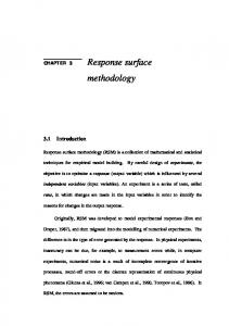
Figure 1: Tilted Ellipsoid Contours E(w | d1 , d 2 ) with Global and Local Experimental Areas In this Monte Carlo experiment we know the truly optimal search direction, namely the vector (say) g that starts at d and ends at the true optimum (0, 0 ).′ So we
COMPARISON OF ASD AND SD THROUGH MONTE CARLO EXPERIMENTS
0
To compare the ASD and SD search directions, we perform Monte Carlo experiments. The Monte Carlo method is an efficient and effective way to estimate the behavior of search techniques applied to random simulations; see Kleijnen et al. (2002). We limit the example to two inputs, so k = 2. We generate the simulation output w through a second-order polynomial with white noise: w = β 0 + β1 d 1 + β 2 d 2 + β1; 1 d 12 + β 2; 2 d 22 + β1; 2 d 1 d 2 + e .
compute the angle (say) θˆ between the true search direction g and the estimated search direction p : θˆ = arccos
g′p . g 2 p2
(8)
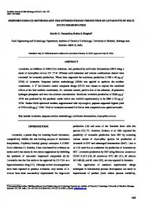
Obviously, the smaller θˆ is, the better the search technique performs. To estimate the distribution of θˆ defined in (8), we
(7)
take 100 macro-replications. Figure 2 shows a bundle of 100 p' s around g when σ e = 0.10. In each macroreplicate, we apply SD and ASD to the same I/O data (w, d , d ). We characterize the resulting empirical θˆ dis-
The response surface (7) holds for the global area, for which we take the unit square: −1 ≤ d 1 ≤ 1 and −1 ≤ d 2 ≤ 1. (We have already seen that RSM fits firstorder polynomials locally.) In the local area we use a one-at-a-time design, because this design is non-orthogonal - and in practice designs in the original inputs are not orthogonal (see Kleijnen et al. (2002)). The specific local area is in the lower corner of Figure 1. To enable the computation of the MSR, we simulate one input combination twice: m1 = 2.
1
2
tribution through several statistics, namely its average, standard deviation, and specific quantiles; see Table 1.
We consider a specific case of (7): β 0 = β1 = β 2 = 0, β1; 2 = 2, β1; 1 = -2, β 2; 2 = -1, so the contour functions (for example, iso-cost curves) form ellipsoids tilted relative to the d 1 and d 2 axes. Hence, (7) has as its true optimum d * = (0, 0 )′ . After fitting a first-order polynomial, we estimate the SD and ASD paths starting from d 0′ = (0.85, -0.95), explained above (4).
Figure 2: 100 ASD Search Directions p and the Truly Optimal Search Direction g (Marked by Thick Dots)
379
Angün, Kleijnen, Den Hertog, and Gürkan Formally, our problem becomes:
Table 1: Statistics in case of Interactions, for ASD and SD’s Estimated Angle Error θˆ (in Degrees) σ e = 0.10 σ e = 0.25 Statistics ASD SD ASD SD Average 9.72 16.01 10.14 17.33 Standard deviation 3.30 6.23 7.69 12.88 Median (50% quantile) 9.68 16.02 8.99 14.94 75% quantile 12.37 21.12 16.13 27.87 25% quantile 6.99 10.76 3.21 5.84 95% quantile 15.66 27.05 24.78 41.55 5% quantile 4.99 6.80 0.61 0.81 100% quantile 17.41 30.08 32.07 50.99 0% quantile 0.85 1.46 0.04 0.25
subject to
E(w h (d )) ≥ a h for h = 1, ..., z − 1
(9)
l ≤d ≤u where d is the vector of simulation inputs, l and u the deterministic lower and upper bounds on d , a h the righthand-side value for the hth constraint, and wh′ (h ′ = 0 , ..., z − 1) is the response h′. Note that probabilities (for example, service percentages) can be formulated as expected values of indicator functions. Further, the multiple simulation responses are correlated, since they are estimated through the same PRN fed into the same simulation model. As in Part 1, we locally fit a first-order polynomial – but now for each response; see (1). However, the noise e is now multi-variate normal – still with zero means but now with covariance matrix (say) Σ . Yet, since the same design is used for all z responses, the GLS estimator reduces to the OLS estimator; see Ruud (2000, p. 703). Therefore we still use (2), but to the symbol βˆ we add the
Further, we perform the Monte Carlo experiment for two noise values: σ e is 0.10 or 0.25. We use the same PRN for both values. In case of high noise, the estimated search directions may be very wrong. Nevertheless, ASD still performs better; see again Table 1. In general, ASD performs better than SD, unless we focus on outliers; see Kleijnen et al. (2002). 4
E(w0 (d ))
minimize
MULTIPLE RESPONSES: INTERIOR POINT AND BINARY SEARCH APPROACH
subscript h′. Further, for h ′, h ′′ = 0, … , z − 1 we estimate Σ through the analogue of (3):
In Part 1, we assumed a single response of interest – denoted by w in (2). Now we consider a more realistic situation, namely the simulation generates multiple outputs. For example, an academic inventory simulation defines w in (2) as the sum of inventory-carrying, ordering, and out-of-stock costs, whereas a practical simulation minimizes the sum of the expected inventory-carrying and ordering costs provided the service probability exceeds a pre-specified value. In RSM, there have been several approaches to multiresponse optimization. Khuri (1996) surveys most of these approaches (including desirability functions, generalized distances, and dual responses). Angün et al. (2002) discusses drawbacks of these approaches. To overcome these drawbacks, we propose the following alternative based on mathematical programming. We select one of the responses as the objective and the remaining (say) z − 1 responses as constraints. The SD search would soon hit the boundary of the feasible area formed by these constraints, and would then creep along this boundary. Instead, our search starts in the interior of the feasible area and avoids the boundary; see Barnes (1986) on Karmarkar’s algorithm for linear programming. Note that our approach has the additional advantage of avoiding areas in which the simulation model is not valid and may even crash.
σˆ h2′, h′′ =
We
( w h′ − yˆ h′ )′ ( w h′′ − yˆ h′′ ) Ν − (k + 1 )
introduce
(h = 1, ..., z - 1)
.
B = (b1 , ..., b z −1 )′ ,
(10)
where
bh
denotes the vector of OLS estimates βˆ -0; h (excluding the intercept βˆ 0; h ) for the hth response. Adding slack vectors s, r, and v , we obtain minimize subject to
d ′b0 Bd − s = c, d + r = u, d − v = l,
(11)
s, r, v ≥ 0 where b0 denotes the vector of OLS estimates βˆ -0; 0 (excluding the intercept βˆ ) for w0 , and c is the vector -0; 0
with components c h = a h − βˆ 0; h (h = 1, ..., z - 1). Through (11) we obtain a local linear approximation for (9). Then using ideas from interior point methods - more specifically the affine scaling method - Angün et al. (2002) derives the following search direction: p = − ( B' S −2 B + R −2 + V −2 ) −1 b0
380
(12)
Angün, Kleijnen, Den Hertog, and Gürkan We formulate pessimistic null-hypotheses; that is, we ‘accept’ an input combination only if it gives a significantly lower objective value and all its z − 1 slacks imply a ‘feasible’ solution. Actually, our interior point method implies that a new slack value is a percentage – say, 20% - of the old slack value; our pessimistic hypotheses make our acceptable area smaller than the original feasible area in (9). After we have run G simulations along the search path, we find a ‘best’ solution - so far. Now we wish to reestimate the search direction p defined in (12). Therefore
where S , R , and V are diagonal matrices with the current estimated slack vectors s , r , v > 0 on the diagonal. Obviously, R and V in (12) are known as soon as the deterministic input d to the simulation is selected; S in (12) is estimated from the simulation output, not from the local approximation. Unlike SD, the search direction (12) is scale independent (the inverse of the matrix within the parentheses in (12) scales and projects the estimated SD direction, −b0 ). Having estimated a search direction for a specific starting point through (12), we must next select a step size. Actually, we run the simulation model for several step sizes in that direction, as follows. First, we compute the maximum step size assuming that the local approximation (11) holds globally:
we again use a resolution-3 design in the k factors. We still use CRN; actually, we take the same seeds as we used for the very first local exploration. We save one (expensive) run by using the best combination found so far, as one of the combinations for the design. We stop the whole search when either the computer budget is exhausted or the search returns to an old combination twice. When the search returns to an old combination for the first time, we use a new set of seeds.
λmax = max {0 , min {λ1 , λ2 , λ3 }} where
5
λ1 = min{(ch − bh′ d * ) /p′bh : h∈ {1, ..., z −1}, p′bh < 0} λ2 = min{(u j − d *j ) / p j : j ∈{1, …, k}, p j > 0}
MONTE CARLO EXPERIMENTS FOR MULTIPLE RSM
Like in Part 1 (§3), we study the novel procedure - explained in §4 - by means of a Monte Carlo example. As in §3, we assume globally valid functions quadratic in two inputs, but now we consider three responses; moreover, we add deterministic ‘box’ constraints for the two inputs:
λ3 = min{(l j − d *j ) / p j : j ∈{1, …, k}, p j < 0}.
To increase the probability of staying within the interior of the feasible region, we take only 80% of λmax as our maximum step size. The subsequent step sizes are inspired by binary search, as follows. We systematically halve the current step size along the search direction. At each step, we select as the best point the one with the minimum value for the simulation objective w0 , provided it is feasible. We stop the search in a particular direction after a user-specified number of iterations (say) G = 3. For details see Angün et al. (2002). For all these steps we use common random numbers (CRN), in order to better test whether the objective improves. Moreover, we test whether the other z − 1 responses remain within the feasible area: we test the slack vector s, introduced in (11). These z tests use ratios instead of absolute differences, to avoid scale dependence. A statistical complication is that these ratios may not have finite moments. Therefore we test their medians (not their means). For these tests we use Monte Carlo sampling, which takes negligible computer time compared with the expensive simulation runs. This Monte Carlo takes (say) K = 1000 samples from the assumed distributions with means and variances estimated through the simulation; in the numerical example of the next section we assume z normal distributions ignoring correlations between these responses. From these Monte Carlo samples we compute slack ratios.
minimize subject to
(
E 5 (d 1 − 1) 2 + (d 2 − 5) 2 + 4d 1 d 2 + e0
( E (d
E (d 1 − 3) 2 1
2
+ d 22
) )≤ 9
)
+ d 1 d 2 + e1 ≤ 4
+ 3 (d 2 + 1.061) 2 + e 2 0 ≤ d 1 ≤ 3, − 2 ≤ d 2 ≤ 1
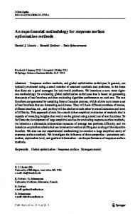
where the noise has σ 0 = 1, σ 1 = 0.15, σ 2 = 0.4, and correlations ρ 0; 1 = 0.6, ρ 0; 2 = 0.3, ρ1; 2 = −0.1. It is easy to derive the analytical solution as * d = (1.24, 0.52)′ with a mean objective value of 22.96 approximately. We select the initial local area shown in the lower left corner of Figure 3. We run 100 macro-replicates; Figure 3 displays the macro-replicate that gives the median result for the objective; that is, 50% of the macro-replicates have worse objective values. In this figure we have dˆ * = (1.46, 0.49)′ and an estimated objective of 25.30 approximately. Table 2 summarizes the 100 macro-replicates, where Criterion 1 is the relative expected objective E w0 d 1* , d 2* − 22.96 /22.96 ; Criteria 2 and 3 stand for
(( (
381
))
)
Angün, Kleijnen, Den Hertog, and Gürkan vised adapted SD (ASD), which corrects for the covariances of the estimated gradient components. ASD is scale independent. Our Monte Carlo experiments demonstrate that - in general - ASD gives a better search direction than SD. In Part 2, we account for multiple simulation responses. We use a mathematical programming approach; that is, we minimize one random objective under random and deterministic constraints. As in classic RSM, we locally fit functions linear in the simulation inputs. Next we apply interior point techniques to these local approximations, to estimate a search direction. This direction is scale independent. We take several steps into this direction, using binary search and statistical tests. Then we re- estimate these local linear functions, etc. Our Monte Carlo experiments demonstrate that our method indeed approaches the true optimum, in relatively few runs with the (expensive) simulation model. Figure 3: The “Average” (50th Quantile) of 100 Estimated Solutions
REFERENCES Angün, E., D. Den Hertog, G. Gürkan, and J. P. C. Kleijnen. 2002. Constrained response surface methodology for simulation with multiple responses. CentER Working Paper. Barnes, E. R. 1986. A variation on Karmarkar’s algorithm for solving linear programming problems. Mathematical Programming 36: 174-182. Box, G. E. P. 1999. Statistics as a catalyst to learning by scientific method, part II - a discussion. Journal of Quality Technology 31 (1): 16-29. Box, G. E. P. and K. B. Wilson. 1951. On the experimental attainment of optimum conditions. Journal of Royal Statistical Society, Series B 13 (1): 1-38. Conn, A. R., N. Gould, and Ph. L. Toint. 2000. Trust Region Methods. Philadelphia: SIAM. Donohue, J. M., E. C. Houck, and R. H. Myers. 1993. Simulation designs and correlation induction for reducing order bias in first-order response surfaces. Operations Research 41 (5): 880-902. --- 1995. Simulation designs for the estimation of response surface gradients in the presence of model misspecification. Management Science 41 (2): 244262. Irizarry, M., J. R. Wilson, and J. Trevino. 2001. A flexible simulation tool for manufacturing-cell design, II: response surface analysis and case study. IIE Transactions 33: 837-846. Khuri, A. I. 1996. Multiresponse surface methodology. In Handbook of Statistics, ed. S. Ghosh and C. R. Rao, 377-406. Amsterdam: Elsevier. Khuri, A. I. and J. A. Cornell. 1996. Response Surfaces: Designs and Analyses. 2d ed. New York: Marcel Dekker.
Table 2: Estimated Objective and Slacks over 100 Macro-replicates Criterion 1 Criterion 2 Criterion 3 10th 0.04 0.03 0.03 quantile th 25 0.06 0.12 0.15 quantile th 50 0.10 0.25 0.29 quantile 75th 0.19 0.43 0.49 quantile 90th 0.18 0.61 0.50 quantile the relative expected slacks
(9 − E(w (d
* 1
* 2
)))
(4 − E(w (d 1
* 1
, d 2*
)))/ 4
and
, d / 9 for the first and the second constraints. Ideally, Criterion 1 is zero; Criteria 2 and 3 are zero if the constraints are binding at the optimum. Our heuristic tends to end at a feasible combination: the table displays only positive quantiles for the Criteria 2 and 3. This feasibility is explained by our pessimistic null hypotheses (and our small significance level α = 0.01 ). Our conclusion is that the heuristic reaches the desired neighborhood of the real optimum in a relatively small number of simulation runs. Once the heuristic reaches this neighborhood, it usually stops at a feasible point. 2
6
CONCLUSIONS
In Part 1 of this paper we addressed the problem of searching for the simulation input combination that minimizes the output. RSM is a classic technique for tackling this problem, but it uses SD, which is scale dependent. Therefore we de-
382
Angün, Kleijnen, Den Hertog, and Gürkan received a number of international fellowships and awards. His e-mail and web address are: and .
Kleijnen, J. P. C. 1993. Simulation and optimization in production planning: a case study. Decision Support Systems 9: 269-280. --- 1998. Experimental design for sensitivity analysis, optimization, and validation of simulation models. In Handbook of Simulation, ed. J. Banks, 173-223. New York: John Wiley & Sons. Kleijnen, J. P. C., D. Den Hertog, and E. Angün. 2002. Response surface methodology’s steepest ascent and step size revisited. CentER Working Paper. Law, A. M. and W. D. Kelton. 2000. Simulation Modeling and Analysis. 3d ed. Boston: McGraw-Hill. Myers, R. H. 1999. Response surface methodology: current status and future directions. Journal of Quality Technology 31 (1): 30-74. Myers, R. H. and D. C. Montgomery. 1995. Response Surface Methodology: Process and Product Optimization Using Designed Experiments. New York: John Wiley & Sons. Neddermeijer, H. G., G. J. van Ootmarsum, N. Piersma, and R. Dekker. 2000. A framework for response surface methodology for simulation optimization models. In Proceedings of the 2000 Winter Simulation Conference, ed. J. A. Joines, R. R. Barton, K. Kang, and P. A. Fishwick, 129-136. Piscataway, New Jersey: Institute of Electrical and Electronics Engineers. Ruud, P. A. 2000. An Introduction to Classical Econometric Theory. New York: Oxford University Press. Safizadeh, M. H. 2002. Minimizing the bias and variance of the gradient estimate in RSM simulation studies. European Journal of Operational Research 136 (1): 121-135. Spall, J. C. 1999. Stochastic optimization and the simultaneous perturbation method. In Proceedings of the 1999 Winter Simulation Conference, ed. P. A. Farrington, H. B. Nembhard, D. T. Sturrock, and G. W. Ewans, 101-109. Piscataway, New Jersey: Institute of Electrical and Electronics Engineers.
DICK DEN HERTOG is a Professor of Operations Research and Management Science at the Center for Economic Research (CentER), within the Faculty of Economics and Business Administration at Tilburg University, in the Netherlands. He received his Ph.D. (cum laude) in 1992. From 1992 until 1999 he was a consultant for optimization at CQM in Eindhoven. His research concerns deterministic and stochastic simulation-based optimization and nonlinear programming, with applications in logistics and production. His e-mail and web address are: and . GÜL GÜRKAN is an Associate Professor of Operations Research and Management Science at the Center for Economic Research (CentER), within the Faculty of Economics and Business Administration at Tilburg University, in the Netherlands. She received her Ph.D. in Industrial Engineering from the University of WisconsinMadison in 1996. Her research interests include simulation, mathematical programming, stochastic optimization, and equilibrium models with applications in logistics, production, telecommunications, economics, and finance. She is a member of INFORMS. Her e-mail and web address are: and
AUTHOR BIOGRAPHIES EBRU ANGÜN is a Ph.D. student at the Department of Information Management at Tilburg University in the Netherlands since 2000. Her e-mail address is . JACK P.C. KLEIJNEN is a Professor of Simulation and Information Systems. His research concerns simulation, mathematical statistics, information systems, and logistics; this research resulted in six books and nearly 200 articles. He has been a consultant for several organizations in the USA and Europe, and has served on many international editorial boards and scientific committees. He spent several years in the USA, at both universities and companies, and
383